2.2.1. Tabulation API Example: Presumed PDF SLFM Tables

This demo is part of Spitfire, with licensing and copyright info here.

Highlights

• Building presumed PDF adiabatic and nonadiabatic SFLM libraries for turbulent flows

• Using Spitfire’s wrapper around the Python interface of `TabProps <https://multiscale.utah.edu/software/>`__ to easily extend tables with clipped Gaussian and Beta PDFs

In this demo, we build reaction models and then incorporate the presumed PDF mixing models outlined in the mixing model documentation.

2.2.1.1. The Reaction Models

First we’ll build the reaction models for an n-heptane/air system following prior demonstrations.

from spitfire import (ChemicalMechanismSpec,
                      Library,
                      FlameletSpec,
                      build_adiabatic_slfm_library,
                      build_nonadiabatic_defect_transient_slfm_library)
import matplotlib.pyplot as plt
import numpy as np

mech = ChemicalMechanismSpec(cantera_input='heptane-liu-hewson-chen-pitsch-highT.yaml',
                             group_name='gas')

pressure = 101325.

air = mech.stream(stp_air=True)
fuel = mech.stream('TPY', (372., pressure, 'NXC7H16:1'))

flamelet_specs = FlameletSpec(mech_spec=mech,
                              initial_condition='equilibrium',
                              oxy_stream=air,
                              fuel_stream=fuel,
                              grid_points=34)

l_ad = build_adiabatic_slfm_library(flamelet_specs,
                                    diss_rate_values=np.logspace(-1, 2, 8),
                                    diss_rate_ref='stoichiometric',
                                    verbose=False)

l_na = build_nonadiabatic_defect_transient_slfm_library(flamelet_specs,
                                                        diss_rate_values=np.logspace(-1, 2, 8),
                                                        diss_rate_ref='stoichiometric',
                                                        n_defect_st=16)

----------------------------------------------------------------------------------
building nonadiabatic (defect) SLFM library
----------------------------------------------------------------------------------
- mechanism: heptane-liu-hewson-chen-pitsch-highT.yaml
- 38 species, 105 reactions
- stoichiometric mixture fraction: 0.062
----------------------------------------------------------------------------------
----------------------------------------------------------------------------------
building adiabatic SLFM library
----------------------------------------------------------------------------------
- mechanism: heptane-liu-hewson-chen-pitsch-highT.yaml
- 38 species, 105 reactions
- stoichiometric mixture fraction: 0.062
----------------------------------------------------------------------------------
   1/   8 (chi_stoich =  1.0e-01 1/s)  converged in   1.06 s, T_max = 2122.1
   2/   8 (chi_stoich =  2.7e-01 1/s)  converged in   0.02 s, T_max = 2089.8
   3/   8 (chi_stoich =  7.2e-01 1/s)  converged in   0.02 s, T_max = 2055.4
   4/   8 (chi_stoich =  1.9e+00 1/s)  converged in   0.08 s, T_max = 2027.5
   5/   8 (chi_stoich =  5.2e+00 1/s)  converged in   0.09 s, T_max = 1984.7
   6/   8 (chi_stoich =  1.4e+01 1/s)  converged in   0.10 s, T_max = 1924.2
   7/   8 (chi_stoich =  3.7e+01 1/s)  converged in   0.10 s, T_max = 1840.6
   8/   8 (chi_stoich =  1.0e+02 1/s)  converged in   0.12 s, T_max = 1695.0
----------------------------------------------------------------------------------
library built in   1.70 s
----------------------------------------------------------------------------------
expanding (transient) enthalpy defect dimension ...
chi_st =  1.0e-01 1/s converged in   3.78 s
chi_st =  2.7e-01 1/s converged in  11.23 s
chi_st =  7.2e-01 1/s converged in   4.64 s
chi_st =  1.9e+00 1/s converged in  10.14 s
chi_st =  5.2e+00 1/s converged in   9.30 s
chi_st =  1.4e+01 1/s converged in   3.14 s
chi_st =  3.7e+01 1/s converged in   3.76 s
chi_st =  1.0e+02 1/s converged in   3.57 s
----------------------------------------------------------------------------------
enthalpy defect dimension expanded in  49.56 s
----------------------------------------------------------------------------------
Structuring enthalpy defect dimension ...
Initializing ... Done.
Interpolating onto structured grid ...
Progress: 0%--10%--20%--30%--40%--50%--60%--70%--80%--100%
Structured enthalpy defect dimension built in   2.30 s
----------------------------------------------------------------------------------
library built in  53.57 s
----------------------------------------------------------------------------------

2.2.1.2. Tabulated Properties

Running a CFD calculation requires fluid properties such as the viscosity, heat capacity, and enthalpy. These are computed on the laminar reaction model and are then integrated with the presumed PDF. So before applying the presumed PDF mixing model we make new libraries with just a few properties likely necessary for the simulation. We typically don’t need to tabulate the entire set of mass fractions, so we’ll remove them to save time.

from spitfire import get_ct_solution_array
import copy

def tabulate_properties(TY_lib):
    ct_sol, lib_shape = get_ct_solution_array(mech, TY_lib)
    prop_lib = copy.copy(TY_lib)
    prop_lib.remove(*prop_lib.props)

    prop_lib['temperature'] = ct_sol.T.reshape(lib_shape)
    prop_lib['viscosity'] = ct_sol.viscosity.reshape(lib_shape)
    prop_lib['enthalpy'] = ct_sol.enthalpy_mass.reshape(lib_shape)
    prop_lib['heat_capacity_cp'] = ct_sol.cp_mass.reshape(lib_shape)

    return prop_lib


prop_ad = tabulate_properties(l_ad)
prop_na = tabulate_properties(l_na)

2.2.1.3. Presumed PDFs

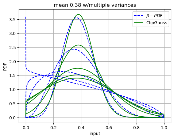
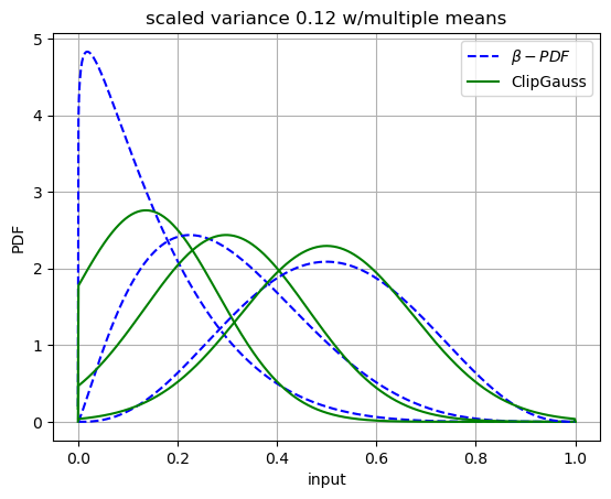
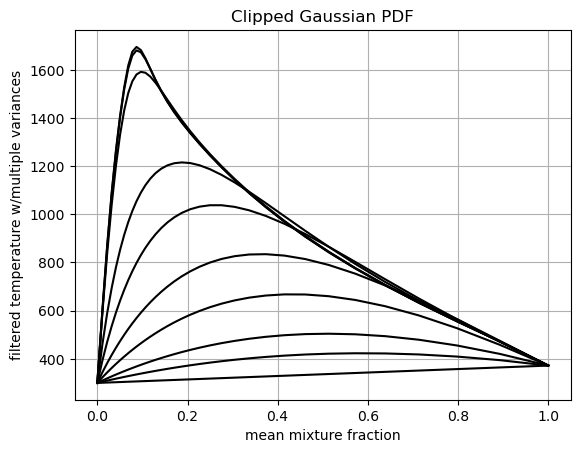
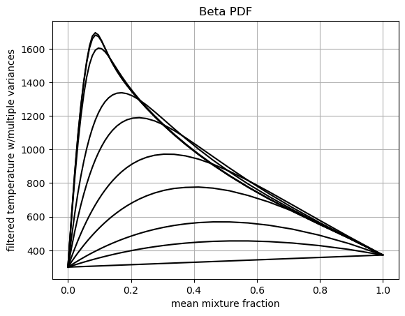
First, we’ll use TabProps to evaluate the clipped Gaussian and \(\beta\) PDFs for some representative means and variances. Note the major differences between the PDF types at higher variances and near the boundaries. The poor behavior of the \(\beta\) PDF in these regimes makes it substantially harder to integrate than the clipped Gaussian.

from spitfire import BetaPDF, ClipGaussPDF

ztest = np.linspace(0, 1, 1000)

cg = ClipGaussPDF()
bp = BetaPDF()

zmean = 0.38
for i, zsvar in enumerate([0.05, 0.1, 0.2, 0.25, 0.28]):
    bp.set_mean(zmean)
    bp.set_scaled_variance(zsvar)
    plt.plot(ztest, bp.get_pdf(ztest), 'b--', label='$\\beta-PDF$' if i == 0 else None)
    cg.set_mean(zmean)
    cg.set_scaled_variance(zsvar)
    plt.plot(ztest, cg.get_pdf(ztest), 'g-', label='ClipGauss' if i == 0 else None)
plt.title(f'mean {zmean:.2f} w/multiple variances')
plt.xlabel('input')
plt.ylabel('PDF')
plt.grid()
plt.legend()
plt.show()

zsvar = 0.12
for i, zmean in enumerate([0.15, 0.3, 0.5]):
    bp.set_mean(zmean)
    bp.set_scaled_variance(zsvar)
    plt.plot(ztest, bp.get_pdf(ztest), 'b--', label='$\\beta-PDF$' if i == 0 else None)
    cg.set_mean(zmean)
    cg.set_scaled_variance(zsvar)
    plt.plot(ztest, cg.get_pdf(ztest), 'g-', label='ClipGauss' if i == 0 else None)
plt.title(f'scaled variance {zsvar:.2f} w/multiple means')
plt.xlabel('input')
plt.ylabel('PDF')
plt.grid()
plt.legend()
plt.show()

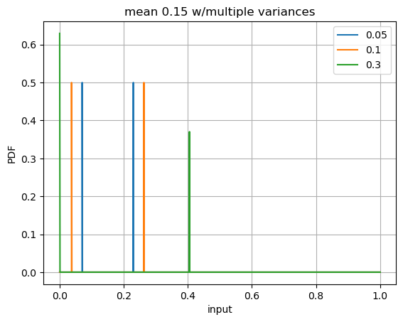
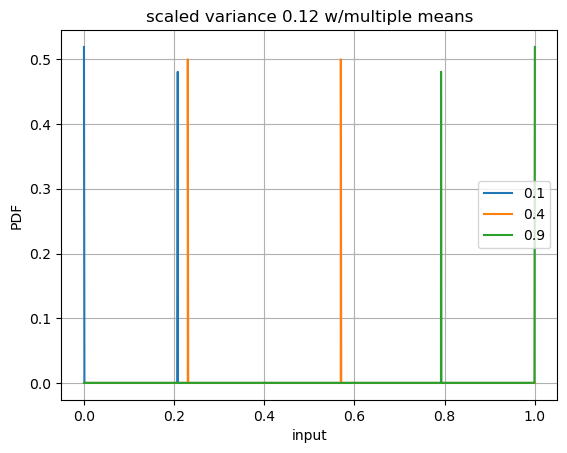
Another PDF supported in Spitfire is a DoubleDeltaPDF shown below. To be precise, what we show below is not the actual double delta PDF but its integral.

from spitfire import DoubleDeltaPDF

ztest = np.linspace(0, 1, 1000)
colors = ['k','r','b']

ddelta = DoubleDeltaPDF()

zmean = 0.15
for i, zsvar in enumerate([0.05, 0.1, 0.3]):
    ddelta.set_mean(zmean)
    ddelta.set_scaled_variance(zsvar)
    nonzero_points = np.array([ddelta.find_bounds()[0],ddelta.find_bounds()[1]])
    zfull = np.sort(np.hstack((ztest, nonzero_points)))
    plt.plot(zfull, ddelta.get_pdf(zfull), '-', label=str(zsvar))
plt.title(f'mean {zmean:.2f} w/multiple variances')
plt.xlabel('input')
plt.ylabel('PDF')
plt.grid()
plt.legend()
plt.show()

zsvar = 0.12
for i, zmean in enumerate([0.1, 0.4, 0.9]):
    ddelta.set_mean(zmean)
    ddelta.set_scaled_variance(zsvar)
    nonzero_points = np.array([ddelta.find_bounds()[0],ddelta.find_bounds()[1]])
    zfull = np.sort(np.hstack((ztest, nonzero_points)))
    plt.plot(zfull, ddelta.get_pdf(zfull), '-', label=str(zmean))
plt.title(f'scaled variance {zsvar:.2f} w/multiple means')
plt.xlabel('input')
plt.ylabel('PDF')
plt.grid()
plt.legend()
plt.show()

2.2.1.4. Incorporating the Mixing Model: PDFs supported by Spitfire

Spitfire provides the apply_mixing_model which takes an existing Library, for instance those computed above, and incorporates subgrid variation for all dimensions and adds the (default) suffix _mean.

Spitfire provides optimized PDF integrators for the following PDFs:

• clipped Gaussian ('ClipGauss')

• \(\beta\) PDF ('Beta')

• double delta PDF ('DoubleDelta')

• delta PDF ('Delta')

Tabprops handles integration of the clipped Gaussian while scipy.integrate.quad handles integration of the Beta PDF. The Delta and DoubleDelta PDF allow for analytic solutions. In addition to these supported PDFs, Spitfire allows you to “roll your own” PDF integrator, a feature to be shown in following demonstrations.

Use mean_values in the PDFSpec to specify an arbitrary (e.g., smaller) grid for the convolutions. The 'Delta' PDF can be used to interpolate the property data onto the mean_values grid.

When calling apply_mixing_model on particularly large laminar libraries, speedup through parallelism can be achieved when num_procs is greater than 1 by setting parallel_type in the PDFSpec to one of the following options:

• 'property': parallelize over properties

• 'property-mean': parallelize over mean and properties

• 'property-variance': parallelize over variance and properties

• 'full': parallelize over mean, variance, and properties

• 'default': use the fastest parallel method on average depending on the pdf

from spitfire import apply_mixing_model, PDFSpec

scaled_variance_values = np.array([0, 0.001, 0.01, 0.1, 0.2, 0.4, 0.6, 0.8, 0.9, 1.0])

mixing_spec = {'mixture_fraction': PDFSpec(pdf='ClipGauss', scaled_variance_values=scaled_variance_values)}

t_cg_prop_ad = apply_mixing_model(prop_ad, mixing_spec, verbose=True)
t_cg_prop_na = apply_mixing_model(prop_na, mixing_spec, verbose=True)

scaled_scalar_variance_mean: computing 10880 integrals...
completed in 2.4 seconds, average = 4560 integrals/s.
scaled_scalar_variance_mean: computing 174080 integrals...
completed in 30.8 seconds, average = 5645 integrals/s.

Now take a quick look at the tables. Input dimensions have been suffixed with _mean and the scalar variance (its scaled form that varies between 0 and 1) is incorporated as the final dimension. Futher, the extra_attributes dictionary that holds library metadata saves the mixing_spec dictionary for later reference.

print(t_cg_prop_ad)
print(t_cg_prop_na)

Spitfire Library with 3 dimensions and 4 properties
------------------------------------------
1. Dimension "mixture_fraction_mean" spanning [0.0, 1.0] with 34 points
2. Dimension "dissipation_rate_stoich_mean" spanning [0.09999999999999999, 100.0] with 8 points
3. Dimension "scaled_scalar_variance_mean" spanning [0.0, 1.0] with 10 points
------------------------------------------
temperature         , min = 299.99999999999994 max = 2122.096955226139
viscosity           , min = 1.2370131775920798e-05 max = 6.906467776683119e-05
enthalpy            , min = -1739935.6849118914 max = 1901.8191601112544
heat_capacity_cp    , min = 1011.3329912202538 max = 2422.2079033534988
Extra attributes: {'mech_spec': <spitfire.chemistry.mechanism.ChemicalMechanismSpec object at 0x7f09512f0d50>, 'mixing_spec': {'mixture_fraction': <spitfire.chemistry.tabulation.PDFSpec object at 0x7f0950d2c7d0>}}
------------------------------------------


Spitfire Library with 4 dimensions and 4 properties
------------------------------------------
1. Dimension "mixture_fraction_mean" spanning [0.0, 1.0] with 34 points
2. Dimension "dissipation_rate_stoich_mean" spanning [0.09999999999999999, 100.0] with 8 points
3. Dimension "enthalpy_defect_stoich_mean" spanning [-2140683.3798015513, 0.0] with 16 points
4. Dimension "scaled_scalar_variance_mean" spanning [0.0, 1.0] with 10 points
------------------------------------------
temperature         , min = 299.99999999999994 max = 2122.096955226139
viscosity           , min = 1.2370131775920718e-05 max = 6.906467776683119e-05
enthalpy            , min = -2521367.43587239 max = 1901.8191601113401
heat_capacity_cp    , min = 1011.3329912202537 max = 2422.2079033534988
Extra attributes: {'mech_spec': <spitfire.chemistry.mechanism.ChemicalMechanismSpec object at 0x7f0950e07850>, 'mixing_spec': {'mixture_fraction': <spitfire.chemistry.tabulation.PDFSpec object at 0x7f0950d2c7d0>}}
------------------------------------------

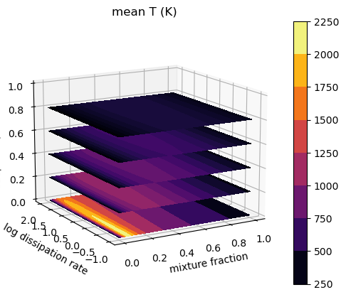
from mpl_toolkits.mplot3d import axes3d
from matplotlib.colors import Normalize

To finish things off we can show some simple visualiations of the data.

fig = plt.figure()
ax = fig.add_subplot(projection='3d')
z = np.squeeze(t_cg_prop_ad.mixture_fraction_mean_grid[:, :, 0])
x = np.squeeze(np.log10(t_cg_prop_ad.dissipation_rate_stoich_mean_grid[:, :, 0]))
v_list = t_cg_prop_ad.scaled_scalar_variance_mean_values
for idx in [7, 6, 5, 4, 0]:
    p = ax.contourf(z, x, np.squeeze(t_cg_prop_ad['temperature'][:, :, idx]),
                    offset=v_list[idx],
                    cmap='inferno',
                    norm=Normalize(300, 2200))
plt.colorbar(p)
ax.view_init(elev=14, azim=-120)
ax.set_zlim([0, 1])
ax.set_xlabel('mixture fraction')
ax.set_ylabel('log dissipation rate')
ax.set_zlabel('scaled scalar variance')
ax.set_title('mean T (K)')
plt.show()

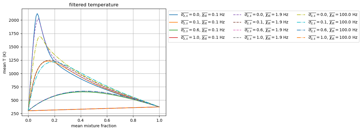
j = 0
chi = t_cg_prop_ad.dissipation_rate_stoich_mean_values[j]
for i in range(0, t_cg_prop_ad.scaled_scalar_variance_mean_npts, 3):
    svar = t_cg_prop_ad.scaled_scalar_variance_mean_values[i]
    plt.plot(t_cg_prop_ad.mixture_fraction_mean_values, np.squeeze(t_cg_prop_ad['temperature'][:, j, i]),
             '-',
             label='$\\overline{\sigma_{z,s}}=$'+f'{svar}'+', $\\overline{\\chi_{\\rm st}}=$'+f'{chi:.1f} Hz')
j = 3
chi = t_cg_prop_ad.dissipation_rate_stoich_mean_values[j]
for i in range(0, t_cg_prop_ad.scaled_scalar_variance_mean_npts, 3):
    svar = t_cg_prop_ad.scaled_scalar_variance_mean_values[i]
    plt.plot(t_cg_prop_ad.mixture_fraction_mean_values, np.squeeze(t_cg_prop_ad['temperature'][:, j, i]),
             '--',
             label='$\\overline{\sigma_{z,s}}=$'+f'{svar}'+', $\\overline{\\chi_{\\rm st}}=$'+f'{chi:.1f} Hz')
j = 7
chi = t_cg_prop_ad.dissipation_rate_stoich_mean_values[j]
for i in range(0, t_cg_prop_ad.scaled_scalar_variance_mean_npts, 3):
    svar = t_cg_prop_ad.scaled_scalar_variance_mean_values[i]
    plt.plot(t_cg_prop_ad.mixture_fraction_mean_values, np.squeeze(t_cg_prop_ad['temperature'][:, j, i]),
             '-.',
             label='$\\overline{\sigma_{z,s}}=$'+f'{svar}'+', $\\overline{\\chi_{\\rm st}}=$'+f'{chi:.1f} Hz')
plt.xlabel('mean mixture fraction')
plt.ylabel('mean T (K)')
plt.title('filtered temperature')
plt.grid()
plt.legend(bbox_to_anchor=(1, 1), loc='upper left', ncol=3)
plt.show()

Below, we compare the convolution of a property using the different supported PDFs. We will pick a single property profile.

prop = 'temperature'
sampled_lib = Library(prop_ad.dims[0])
sampled_lib[prop] = Library.copy(prop_ad)[prop][:,-1]

t_cg_T_ad = apply_mixing_model(sampled_lib, {'mixture_fraction': PDFSpec(pdf='ClipGauss', scaled_variance_values=scaled_variance_values)}, verbose=True)
t_bp_T_ad = apply_mixing_model(sampled_lib, {'mixture_fraction': PDFSpec(pdf='Beta', scaled_variance_values=scaled_variance_values)}, verbose=True)
t_dd_T_ad = apply_mixing_model(sampled_lib, {'mixture_fraction': PDFSpec(pdf='DoubleDelta', scaled_variance_values=scaled_variance_values)}, verbose=True)

scaled_scalar_variance_mean: computing 340 integrals...
completed in 0.3 seconds, average = 1299 integrals/s.
scaled_scalar_variance_mean: computing 340 integrals...
completed in 3.6 seconds, average = 93 integrals/s.
scaled_scalar_variance_mean: computing 340 integrals...
completed in 0.0 seconds, average = 12779 integrals/s.

for i in range(scaled_variance_values.size):
    plt.plot(t_cg_T_ad.mixture_fraction_mean_values, t_cg_T_ad[prop][:, i], 'k-')
plt.xlabel('mean mixture fraction')
plt.ylabel('filtered '+prop+' w/multiple variances')
plt.title('Clipped Gaussian PDF')
plt.grid()
plt.show()

for i in range(scaled_variance_values.size):
    plt.plot(t_bp_T_ad.mixture_fraction_mean_values, t_bp_T_ad[prop][:, i], 'k-')
plt.xlabel('mean mixture fraction')
plt.ylabel('filtered '+prop+' w/multiple variances')
plt.title('Beta PDF')
plt.grid()
plt.show()

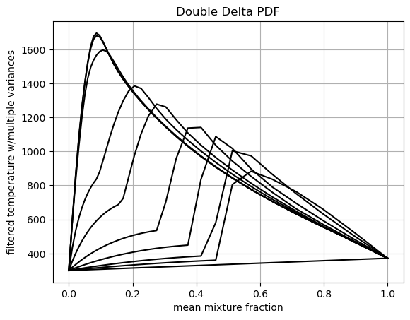
for i in range(scaled_variance_values.size):
    plt.plot(t_dd_T_ad.mixture_fraction_mean_values, t_dd_T_ad[prop][:, i], 'k-')
plt.xlabel('mean mixture fraction')
plt.ylabel('filtered '+prop+' w/multiple variances')
plt.title('Double Delta PDF')
plt.grid()
plt.show()

Below is an example of using the delta PDF to interpolate onto a smaller grid.

smaller_lib = apply_mixing_model(sampled_lib, {'mixture_fraction': PDFSpec(pdf='delta', mean_values=sampled_lib.mixture_fraction_values[::2])}, verbose=True)
print('temperature difference between original and subsampled libraries:',np.max(np.abs(smaller_lib['temperature'] - sampled_lib['temperature'][::2])))
print('original library size:', sampled_lib.shape)
print('subsampled library size:', smaller_lib.shape)

scaled_scalar_variance_mean: computing 17 integrals...
completed in 0.0 seconds, average = 5476 integrals/s.
temperature difference between original and subsampled libraries: 2.2737367544323206e-13
original library size: (34,)
subsampled library size: (17,)

All PDFs, \(P(\phi)\), must satisfy the following integrals:

1. \(1 = \int_{-\infty}^\infty P(\phi) \mathrm{d}\phi\)

2. \(\bar{\phi} = \int_{-\infty}^\infty \phi P(\phi) \mathrm{d}\phi\)

3. \(\sigma_{\phi}^2 = \int_{-\infty}^\infty (\phi - \bar{\phi})^2 P(\phi) \mathrm{d}\phi\)

Spitfire provides the function compute_pdf_max_integration_errors for computing the relative errors in satisfying those integrals. This is useful when determining acceptable parameters for the \(\beta\)-PDF, for example. Below we show the relative errors using the default values for the BetaPDF parameters.

from spitfire import compute_pdf_max_integration_errors

svars = np.array([0., 1.e-5, 6.e-4, 1.e-3, 0.1, 0.5, 0.8, 0.86, 0.9, 0.95, 1.])
means = np.hstack((0,np.logspace(-5,0,100)))

pdf = BetaPDF(scaled_variance_max_integrate=0.86,
              scaled_variance_min_integrate=6.e-4,
              mean_boundary_integrate=6.e-5)

print(compute_pdf_max_integration_errors(pdf, means, svars))

(0.000591317734758956, 2.4555011311778803e-06, 0.009900892069395255)