4.2.7. Implicit time integration basics
This demo is part of Spitfire, with licensing and copyright info here.
Highlights
a basic example of the implicit Backward Euler method of solving a simple differential equation
4.2.7.1. Introduction
This notebook demonstrates the use of Spitfire’s implicit time
integration methods for solving the simple exponential decay problem
introduced in other notebooks. The default behavior of the odesolve
method presented earlier is in fact to use an implicit method - these
demonstrations show how to go beyond the default behavior.
Following prior demonstrations, we import some useful classes, set up the problem, and solve first with Forward Euler as before.
import numpy as np
from spitfire import odesolve, ForwardEulerS1P1

dt = 0.05
tf = 1.0
k = -10.
y0 = np.array([1.])

rhs = lambda t, y: k * y

output_times = np.linspace(0., tf, 21)

y_fe = odesolve(rhs, y0, output_times, step_size=dt, method=ForwardEulerS1P1())
To solve with the implicit Backward Euler method, we import the
BackwardEulerS1P1Q1 and SimpleNewtonSolver classes.
BackwardEulerS1P1Q1 is the time stepper class and
SimpleNewtonSolver will be the underlying solver for the nonlinear
system of equations solved in each time step.
Note from the output of integrate in this case that we now have
nontrivial numbers for the nonlinear iter, linear iter, and
Jacobian setups fields. These aren’t particularly interesting in
this case because the exponential decay problem is linear and we haven’t
set up any advanced solution options. We’ll cover these in a later
notebook.
The only distinction between using this implicit method and the explicit
methods used before is that the BackwardEulerS1P1Q1 instance is
built with a SimpleNewtonSolver object when passed to integrate.
This simplicity is present in this case because we are letting Spitfire
use a default dense linear solver (LU factorization and
back-substitution with LAPACK) and a finite difference approximation to
the Jacobian matrix of the system. In cases where a dense solver and
approximate Jacobian matrix are appropriate, this is a very convenient
option. However, in many cases of practical interest this is not
efficient and more advanced options need to be explored - these will be
covered in later demonstrations.
from spitfire import BackwardEulerS1P1Q1, SimpleNewtonSolver

y_be = odesolve(rhs, y0, output_times, step_size=dt, method=BackwardEulerS1P1Q1(SimpleNewtonSolver()))
Now we can just as easily use the more advanced
KennedyCarpenterS6P4Q3 method. This method is the workhorse of
Spitfire’s solvers for complex chemistry problems and is extremely
useful as a general solver - it is the default method used by
odesolve along with adaptive time-stepping not shown here. It is
fourth-order accurate and possesses excellent characteristics such as
L-stability, a stage order of two (due to the explicit first stage), and
singly diagonally implicit solves meaning that its embedded linear
systems may be solved much more efficiently than those of fully implicit
Runge-Kutta methods with comparable properties.
from spitfire import KennedyCarpenterS6P4Q3

y_esdirk64 = odesolve(rhs, y0, output_times, step_size=dt, method=KennedyCarpenterS6P4Q3(SimpleNewtonSolver()))
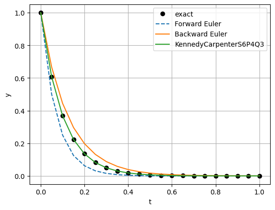
Plotting the solutions from the Forward and Backward Euler methods along with the exact solution shows that the two methods yield exactly opposite errors. When the nonlinear system in Backward Euler’s time steps can be solved exactly this is consistent with theory. This also shows that the Runge Kutta method is exceptionally accurate.
import matplotlib.pyplot as plt

plt.plot(output_times, y0 * np.exp(k * output_times), 'ko', label='exact')
plt.plot(output_times, y_fe, '--', label='Forward Euler')
plt.plot(output_times, y_be, '-', label='Backward Euler')
plt.plot(output_times, y_esdirk64, '-', label='KennedyCarpenterS6P4Q3')

plt.xlabel('t')
plt.ylabel('y')
plt.legend(loc='best')
plt.grid()
plt.show()
4.2.7.2. Conclusions
This notebook shows the simplest use of some implicit time-stepping methods, including a high-order Runge-Kutta method, with Spitfire. Implicit methods can perform extremely well for many classes of problems when fine-tuned - examples of such fine-tuning will follow in more advanced demonstrations.