2.9. Tabulation API Example: Nonadiabatic Flamelet Models
This demo is part of Spitfire, withlicensing and copyright info here.
Highlights - using build_nonadiabatic* methods in Spitfire to
build nonadiabatic equilibrium, Burke-Schumann, and SLFM models
This example builds nonadiabatic flamelet models and compares profiles of the temperature, mass fractions, and enthalpy defect of several nonadiabatic flamelet tabulation techniques for n-heptane chemistry.
from spitfire import (ChemicalMechanismSpec,
                      FlameletSpec,
                      build_nonadiabatic_defect_eq_library,
                      build_nonadiabatic_defect_bs_library,
                      build_nonadiabatic_defect_transient_slfm_library,
                      build_nonadiabatic_defect_steady_slfm_library)
import matplotlib.pyplot as plt
import numpy as np

mech = ChemicalMechanismSpec(cantera_xml='heptane-liu-hewson-chen-pitsch-highT.xml', group_name='gas')
pressure = 101325.
air = mech.stream(stp_air=True)
air.TP = 300., pressure
fuel = mech.stream('TPX', (485., pressure, 'NXC7H16:1'))

flamelet_specs = {'mech_spec': mech, 'oxy_stream': air, 'fuel_stream': fuel, 'grid_points': 128}
l_eq = build_nonadiabatic_defect_eq_library(FlameletSpec(**flamelet_specs), verbose=False)
l_bs = build_nonadiabatic_defect_bs_library(FlameletSpec(**flamelet_specs), verbose=False)
l_ts = build_nonadiabatic_defect_transient_slfm_library(FlameletSpec(**flamelet_specs),
                                                        verbose=True,
                                                        diss_rate_values=np.array([1e-2, 1e-1, 1e0, 1e1, 1e2]),
                                                        diss_rate_log_scaled=True)
----------------------------------------------------------------------------------
building nonadiabatic (defect) SLFM library
----------------------------------------------------------------------------------
- mechanism: heptane-liu-hewson-chen-pitsch-highT.xml
- 38 species, 105 reactions
- stoichiometric mixture fraction: 0.062
----------------------------------------------------------------------------------
----------------------------------------------------------------------------------
building adiabatic SLFM library
----------------------------------------------------------------------------------
- mechanism: heptane-liu-hewson-chen-pitsch-highT.xml
- 38 species, 105 reactions
- stoichiometric mixture fraction: 0.062
----------------------------------------------------------------------------------
   1/   5 (chi_stoich =  1.0e-02 1/s)  converged in   7.67 s, T_max = 2249.2
   2/   5 (chi_stoich =  1.0e-01 1/s)  converged in   0.52 s, T_max = 2186.1
   3/   5 (chi_stoich =  1.0e+00 1/s)  converged in   1.46 s, T_max = 2109.4
   4/   5 (chi_stoich =  1.0e+01 1/s)  converged in   3.72 s, T_max = 1998.4
   5/   5 (chi_stoich =  1.0e+02 1/s)  converged in   0.18 s, T_max = 1768.7
----------------------------------------------------------------------------------
library built in  13.91 s
----------------------------------------------------------------------------------
expanding (transient) enthalpy defect dimension ...
chi_st =  1.0e-02 1/s converged in  20.59 s
chi_st =  1.0e-01 1/s converged in  19.66 s
chi_st =  1.0e+00 1/s converged in  16.75 s
chi_st =  1.0e+01 1/s converged in  14.22 s
chi_st =  1.0e+02 1/s converged in  12.63 s
----------------------------------------------------------------------------------
enthalpy defect dimension expanded in  83.85 s
----------------------------------------------------------------------------------
Structuring enthalpy defect dimension ...
Initializing ... Done.
Interpolating onto structured grid ...
Progress: 0%--10%--20%--30%--40%--50%--100%
Structured enthalpy defect dimension built in   9.68 s
----------------------------------------------------------------------------------
library built in 107.46 s
----------------------------------------------------------------------------------
l_ss = build_nonadiabatic_defect_steady_slfm_library(FlameletSpec(**flamelet_specs),
                                                     verbose=True,
                                                     diss_rate_values=np.array([1e-2, 1e-1, 1e0, 1e1, 1e2]),
                                                     diss_rate_log_scaled=True,
                                                     solver_verbose=False,
                                                     h_stoich_spacing=1.e-3)
----------------------------------------------------------------------------------
building nonadiabatic (defect) SLFM library
----------------------------------------------------------------------------------
- mechanism: heptane-liu-hewson-chen-pitsch-highT.xml
- 38 species, 105 reactions
- stoichiometric mixture fraction: 0.062
----------------------------------------------------------------------------------
----------------------------------------------------------------------------------
building adiabatic SLFM library
----------------------------------------------------------------------------------
- mechanism: heptane-liu-hewson-chen-pitsch-highT.xml
- 38 species, 105 reactions
- stoichiometric mixture fraction: 0.062
----------------------------------------------------------------------------------
   1/   5 (chi_stoich =  1.0e-02 1/s)  converged in   7.15 s, T_max = 2249.2
   2/   5 (chi_stoich =  1.0e-01 1/s)  converged in   0.45 s, T_max = 2186.1
   3/   5 (chi_stoich =  1.0e+00 1/s)  converged in   1.41 s, T_max = 2109.4
   4/   5 (chi_stoich =  1.0e+01 1/s)  converged in   3.27 s, T_max = 1998.4
   5/   5 (chi_stoich =  1.0e+02 1/s)  converged in   0.17 s, T_max = 1768.7
----------------------------------------------------------------------------------
library built in  12.83 s
----------------------------------------------------------------------------------
expanding (steady) enthalpy defect dimension ...
chi_st =  1.0e-02 1/s converged in 124.93 s
chi_st =  1.0e-01 1/s converged in  47.30 s
chi_st =  1.0e+00 1/s converged in  27.73 s
chi_st =  1.0e+01 1/s converged in  19.77 s
chi_st =  1.0e+02 1/s converged in  35.97 s
----------------------------------------------------------------------------------
enthalpy defect dimension expanded in 255.75 s
----------------------------------------------------------------------------------
Structuring enthalpy defect dimension ...
Initializing ... Done.
Interpolating onto structured grid ...
Progress: 0%--10%--20%--30%--40%--50%--100%
Structured enthalpy defect dimension built in  10.35 s
----------------------------------------------------------------------------------
library built in 278.96 s
----------------------------------------------------------------------------------
c_ts = 'SpringGreen'
c_ss = 'Indigo'
c_eq = 'DodgerBlue'
c_bs = 'DarkOrange'
ichi1 = 1
ichi2 = 4
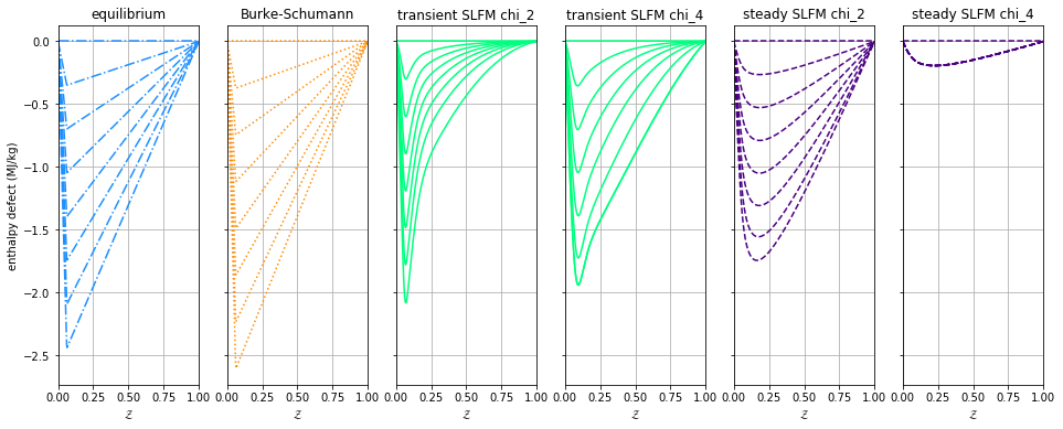
fig, axarray = plt.subplots(1, 6, sharex=True, sharey=True)
axarray[0].plot(l_eq.mixture_fraction_values, l_eq['enthalpy_defect'][:, ::2] * 1e-6, '-.', color=c_eq)
axarray[1].plot(l_bs.mixture_fraction_values, l_bs['enthalpy_defect'][:, ::2] * 1e-6, ':', color=c_bs)
axarray[2].plot(l_ts.mixture_fraction_values, l_ts['enthalpy_defect'][:, ichi1, ::4] * 1e-6, '-', color=c_ts)
axarray[3].plot(l_ts.mixture_fraction_values, l_ts['enthalpy_defect'][:, ichi2, ::4] * 1e-6, '-', color=c_ts)
axarray[4].plot(l_ss.mixture_fraction_values, l_ss['enthalpy_defect'][:, ichi1, ::4] * 1e-6, '--', color=c_ss)
axarray[5].plot(l_ss.mixture_fraction_values, l_ss['enthalpy_defect'][:, ichi2, ::4] * 1e-6, '--', color=c_ss)
axarray[0].set_ylabel('enthalpy defect (MJ/kg)')
axarray[0].set_title('equilibrium')
axarray[1].set_title('Burke-Schumann')
axarray[2].set_title('transient SLFM chi_2')
axarray[3].set_title('transient SLFM chi_4')
axarray[4].set_title('steady SLFM chi_2')
axarray[5].set_title('steady SLFM chi_4')
for ax in axarray:
ax.set_xlim([0, 1])
ax.grid()
ax.set_xlabel('$\\mathcal{Z}$')
fig.set_size_inches(16, 6)
plt.show()
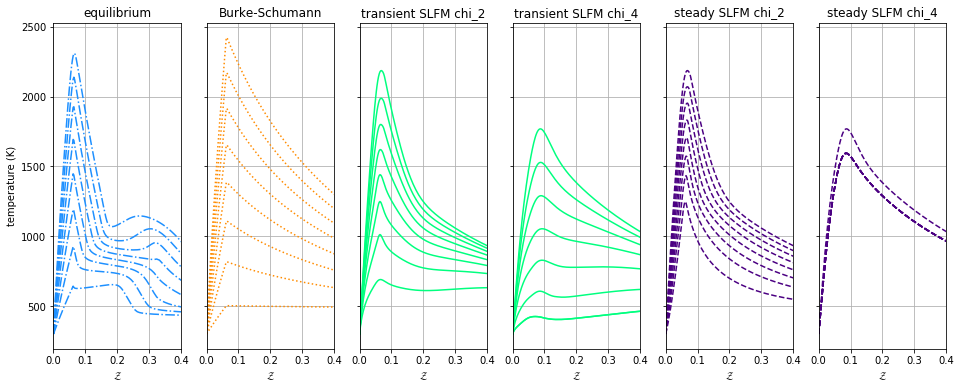
fig, axarray = plt.subplots(1, 6, sharex=True, sharey=True)
axarray[0].plot(l_eq.mixture_fraction_values, l_eq['temperature'][:, ::2], '-.', color=c_eq)
axarray[1].plot(l_bs.mixture_fraction_values, l_bs['temperature'][:, ::2], ':', color=c_bs)
axarray[2].plot(l_ts.mixture_fraction_values, l_ts['temperature'][:, ichi1, ::4], '-', color=c_ts)
axarray[3].plot(l_ts.mixture_fraction_values, l_ts['temperature'][:, ichi2, ::4], '-', color=c_ts)
axarray[4].plot(l_ss.mixture_fraction_values, l_ss['temperature'][:, ichi1, ::4], '--', color=c_ss)
axarray[5].plot(l_ss.mixture_fraction_values, l_ss['temperature'][:, ichi2, ::4], '--', color=c_ss)
axarray[0].set_ylabel('temperature (K)')
axarray[0].set_title('equilibrium')
axarray[1].set_title('Burke-Schumann')
axarray[2].set_title('transient SLFM chi_2')
axarray[3].set_title('transient SLFM chi_4')
axarray[4].set_title('steady SLFM chi_2')
axarray[5].set_title('steady SLFM chi_4')
for ax in axarray:
ax.set_xlim([0, 0.4])
ax.grid()
ax.set_xlabel('$\\mathcal{Z}$')
fig.set_size_inches(16, 6)
plt.show()
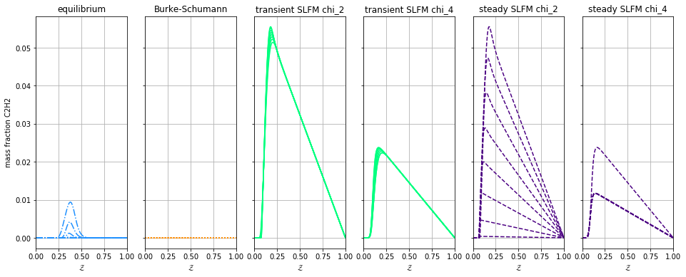
fig, axarray = plt.subplots(1, 6, sharex=True, sharey=True)
axarray[0].plot(l_eq.mixture_fraction_values, l_eq['mass fraction C2H2'][:, ::2], '-.', color=c_eq)
axarray[1].plot(l_bs.mixture_fraction_values, l_bs['mass fraction C2H2'][:, ::2], ':', color=c_bs)
axarray[2].plot(l_ts.mixture_fraction_values, l_ts['mass fraction C2H2'][:, ichi1, ::4], '-', color=c_ts)
axarray[3].plot(l_ts.mixture_fraction_values, l_ts['mass fraction C2H2'][:, ichi2, ::4], '-', color=c_ts)
axarray[4].plot(l_ss.mixture_fraction_values, l_ss['mass fraction C2H2'][:, ichi1, ::4], '--', color=c_ss)
axarray[5].plot(l_ss.mixture_fraction_values, l_ss['mass fraction C2H2'][:, ichi2, ::4], '--', color=c_ss)
axarray[0].set_ylabel('temperature (K)')
axarray[0].set_title('equilibrium')
axarray[1].set_title('Burke-Schumann')
axarray[2].set_title('transient SLFM chi_2')
axarray[3].set_title('transient SLFM chi_4')
axarray[4].set_title('steady SLFM chi_2')
axarray[5].set_title('steady SLFM chi_4')
axarray[0].set_ylabel('mass fraction C2H2')
for ax in axarray:
ax.set_xlim([0, 1])
ax.grid()
ax.set_xlabel('$\\mathcal{Z}$')
fig.set_size_inches(16, 6)
plt.show()
from mpl_toolkits.mplot3d import axes3d
from matplotlib.colors import Normalize

fig = plt.figure()
ax = fig.gca(projection='3d')
z = l_ts.mixture_fraction_grid[:, :, 0]
x = np.log10(l_ts.dissipation_rate_stoich_grid[:, :, 0])
for ih in range(0, l_ts.enthalpy_defect_stoich_npts, 6):
    dh = l_ts.enthalpy_defect_stoich_values[ih]
    ax.contourf(z, x, l_ts['temperature'][:, :, ih], offset=dh / 1.e6,
                cmap='inferno', levels=30, norm=Normalize(vmin=300, vmax=2400))
ax.set_zlim([0, 0.7])
ax.set_xlabel('$\\mathcal{Z}$')
ax.set_ylabel('$\\log_{10}\\chi_{\\rm st}$ (Hz)')
ax.set_zlabel('$\\gamma$ (MJ/kg)')
ax.set_zticks([-2.0, -1.5, -1.0, -0.5, 0.0])
ax.set_title('gas temperature (K)')
fig.set_size_inches(8, 8)
plt.show()

fig = plt.figure()
ax = fig.gca(projection='3d')
for ih in range(0, l_ts.enthalpy_defect_stoich_npts, 6):
    dh = l_ts.enthalpy_defect_stoich_values[ih]
    ax.contourf(z, x, l_ts['mass fraction OH'][:, :, ih], offset=dh / 1.e6,
                cmap='Oranges', levels=30, norm=Normalize(vmin=0, vmax=5e-3), alpha=0.8)
ax.set_zlim([0, 0.7])
ax.set_xlabel('$\\mathcal{Z}$')
ax.set_ylabel('$\\log_{10}\\chi_{\\rm st}$ (Hz)')
ax.set_zlabel('$\\gamma$ (MJ/kg)')
ax.set_zticks([-2.0, -1.5, -1.0, -0.5, 0.0])
ax.set_xlim([0, 0.2])
ax.set_title('mass fraction OH')
fig.set_size_inches(8, 8)
plt.show()
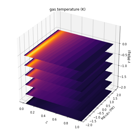
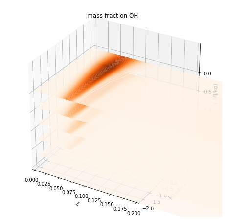
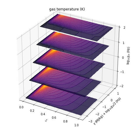
fig = plt.figure()
ax = fig.gca(projection='3d')
z = l_ts.mixture_fraction_grid[:, 0, :]
g = l_ts.enthalpy_defect_stoich_grid[:, 0, :] / 1.e6
for ichi in range(0, l_ts.dissipation_rate_stoich_npts):
    lchi = np.log10(l_ts.dissipation_rate_stoich_values[ichi])
    ax.contourf(z, g + lchi/2, l_ts['temperature'][:, ichi, :], offset=lchi,
                cmap='inferno', levels=30, norm=Normalize(vmin=300, vmax=2400), alpha=0.8)
ax.set_zlim([0, 0.7])
ax.set_xlabel('$\\mathcal{Z}$')
ax.set_ylabel('$\\gamma$ (MJ/kg) + $\\log_{10}\\chi_{\\rm st}/2$ (Hz)')
ax.set_zlabel('$\\log_{10}\\chi_{\\rm st}$ (Hz)')
ax.set_zticks([-2, -1, 0, 1, 2])
ax.set_title('gas temperature (K)')
fig.set_size_inches(8, 8)
plt.show()