4.2.3. Adaptive step size and custom stopping criteria for cannonball trajectories

This demo is part of Spitfire, with licensing and copyright info here.

Highlights

• using adaptive time-stepping to solve nonlinear problems

• defining a custom stopping rule to automatically stop time-stepping when the cannonball has landed

4.2.3.1. Introduction

This example solves for the trajectories of cannonballs launched with drag effects that make the problem nonlinear. The governing equations for the positions and velocities in the \(x\) and \(y\) directions, respectively, are

(4.6)\[\begin{split}\frac{\mathrm{d}}{\mathrm{d}t} \begin{pmatrix} x \\ y \\ v_x \\ v_y \end{pmatrix} = \begin{pmatrix} v_x \\ v_y \\ -\frac{1}{2}\rho_f C_d \frac{A}{\rho V} v_x^2 \\ -g - \frac{1}{2}\rho_f C_d \frac{A}{\rho V} v_y^2 \end{pmatrix}\end{split}\]

where \(g\) is the gravitational acceleration constant, \(C_d\) is the drag coefficient, \(\rho_f\) is the air density, \(\rho\) is the cannonball density, and \(A=4\pi r^2\) and \(V=4/3 \pi r^3\) are the surface area and volume of the cannonball which has radius \(r\). We’re ignoring the effects of buoyancy in this example we’re modeling cannonballs in air and the density difference is large enough.

Solving this system of equations in Spitfire uses largely the same classes and methods already presented in other notebooks. We’ll start by defining the right-hand side as a function of time and the solution vector. We include the drag coefficient in the first method defined, ode_rhs, so that we can more easily modify it to study the effects of drag. Given a value of c_d we’ll write a lambda to provide the Governor a function of time and the solution vector alone.

import numpy as np

rf = 1.23                         # fluid density, kg/m3
ro = 7.86e3                       # object (cannonball) density, kg/m3
g = 9.8                           # gravitational constant, m/s2
r = 4. * 2.54 / 100.              # cannonball radius, m
A = 4. * np.pi * r * r            # surface area, m2
V = np.pi * r * r * r * 4. / 3.   # volume, m3

def ode_rhs(t, q, c_d):
    vel_x = q[2]
    vel_y = q[3]

    f = 0.5 * rf * c_d * A / (ro * V)

    return np.array([vel_x,
                     vel_y,
                     -f * vel_x * vel_x,
                     -g - f * vel_y * vel_y])

4.2.3.2. Custom stopping criteria: stopping when the cannonball lands

The next task is to make a custom stopping rule - we only want to integrate in time until the cannonball has landed. To facilitate this we write a function of the state vector that returns True when the integration should stop. The function below checks that the object’s center is lower than its radius off of the ground and that it currently is falling to the ground with negative \(y\)-velocity (otherwise the laungh point would be caught immediately).

Inside odesolve the stopping criteria is called as

stop_criteria(current_time, current_state, residual, number_of_time_steps)

where residual is the norm of the right-hand side (meant to be used to stop at steady state when the system has stopped evolving) and the other arguments should be fairly clear. It is important that your custom rule takes these arguments in the order above. You can use *args and **kwargs as below, however, to simplify things.

def object_has_landed(t, state, *args, **kwargs):
    vel_y = state[1]
    pos_y = state[3]
    return pos_y < r and vel_y < 0

To use the custom stopping criteria we pass it to the stop_criteria keyword argument of odesolve.

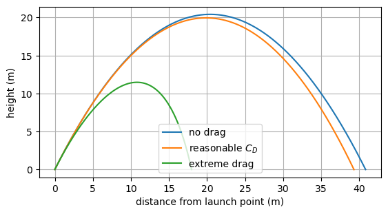
Now we solve the problem for several values of the drag coefficient and plot the results. First we use the classical fourth-order Runge-Kutta method with a constant time step, chosen simply by guessing what might be an appropriate value.

from spitfire import odesolve, RK4ClassicalS4P4
import matplotlib.pyplot as plt

drag_coeff_dict = {'no drag': 0.0, 'reasonable $C_D$': 0.5, 'extreme drag': 20.}

q0 = np.array([0., 0., 10., 20.])  # initial condition

for key in drag_coeff_dict:
    c_d = drag_coeff_dict[key]

    t, q = odesolve(lambda t, y: ode_rhs(t, y, c_d),
                    q0,
                    save_each_step=True,
                    step_size=1.e-3,
                    method=RK4ClassicalS4P4(),
                    stop_criteria=object_has_landed)
    plt.plot(q[:, 0], q[:, 1], label=key)

plt.axis('scaled')
plt.xlabel('distance from launch point (m)')
plt.ylabel('height (m)')
plt.grid()
plt.legend(loc='best')
plt.show()

4.2.3.3. Adaptive time-stepping

Above we had to guess at a value for the time step. Choosing a time step of one millisecond works well enough, but if we choose \(\Delta t=0.1\,s\), which doesn’t sound particularly unreasonable, the methods fail to stop near the point of impact.

A key aspect of effective differential equation solvers is adaptive time-stepping, which is commonly (and in Spitfire) performed with error-control techniques. These techniques use embedded error estimation, meaning low-cast methods of assessing how accurate the solution is (locally). Methods for doing this exist in both linear multistep and Runge-Kutta methods.

Spitfire provides several methods with error estimates to enable adaptive time-stepping, for which a PI controller is available to adapt the time step to maintain the error near a particular target. Next we use the well-known CashKarpS6P5Q4 method (see [https://en.wikipedia.org/wiki/Cash–Karp_method]) and the PI controller to solve the problem without having to choose an arbitrary time step. We do initialize the time step size to a guessed value, although this is typically far easier to do than pick a fixed step size for the entire simulation. We also explicitly provide the target error for the controller and a maximum step size in this case.

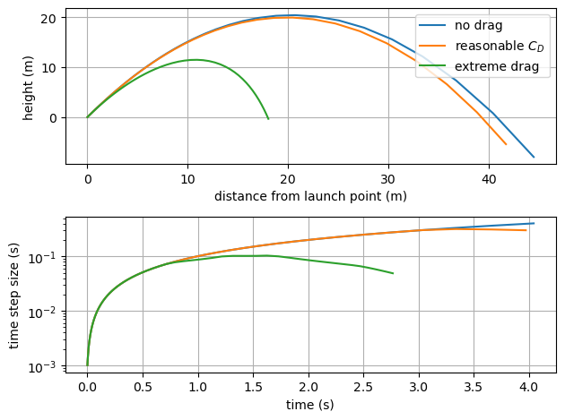
The trajectory plot shows that the solutions are at least reasonable and that the time step is varied quite differently for the case with extreme drag that is particularly nonlinear near the impact point. In the drag-free case the time step simply ramps up to the maximum value, while the other cases see the step size decrease as the object is nearing the ground and the acceleration is increasing (higher \(y\)-velocity magnitude leading to stronger drag forces).

from spitfire import CashKarpS6P5Q4, PIController

figure, axarray = plt.subplots(2, 1)

for key in drag_coeff_dict:
    c_d = drag_coeff_dict[key]

    t, q = odesolve(lambda t, y: ode_rhs(t, y, c_d),
                    q0,
                    save_each_step=True,
                    step_size=PIController(target_error=1.e-8, first_step=1.e-3, max_step=1.e0),
                    method=CashKarpS6P5Q4(),
                    stop_criteria=object_has_landed)
    dt = t[1:] - t[:-1]
    axarray[0].plot(q[:, 0], q[:, 1], label=key)
    axarray[1].semilogy(t[:-1], dt)

axarray[0].set_xlabel('distance from launch point (m)')
axarray[0].set_ylabel('height (m)')
axarray[1].set_xlabel('time (s)')
axarray[1].set_ylabel('time step size (s)')
for ax in axarray:
    ax.grid()
axarray[0].legend(loc='best')
plt.tight_layout()
plt.show()

4.2.3.4. Conclusion

This notebook has shown how to construct user-defined termination rules and use adaptive time-stepping to solve problems where simply guessing a fixed time step size or final simulation time are infeasible or inefficient. Adaptive time-stepping is helpful in solving nonlinear and stiff problems, and it is a key ingredient of Spitfire’s solvers for complex chemistry problems that will be covered later.