1.2.13. Transient Flamelet Example: Ignition Sensitivity to Rate Parameter

This demo is part of Spitfire, with licensing and copyright info here.

Highlights

• Solving transient flamelet ignition trajectories

• Observing sensitivity of the ignition behavior to a key reaction rate parameter

In this demonstration we use the integrate_to_steady method as in previous notebooks, this time to look at how ignition behavior is affected by the pre-exponential factor of a key chain-branching reaction in hydrogen-air ignition. Cantera is used to load the nominal chemistry and modify the reaction rate accordingly.

import cantera as ct
from spitfire import ChemicalMechanismSpec, Flamelet, FlameletSpec
import matplotlib.pyplot as plt
import numpy as np

sol = ct.Solution('h2-burke.yaml', 'h2-burke')

Tair = 1200.
pressure = 101325.
zstoich = 0.1
chi_max = 1.e3
npts_interior = 32

k1mult_list = [0.02, 0.1, 0.2, 1.0, 10.0, 100.0]
sol_dict = dict()

max_time = 0.
max_temp = 0.

A0_original = np.copy(sol.reaction(0).rate.pre_exponential_factor)

for i, k1mult in enumerate(k1mult_list):
    print(f'running {k1mult:.2f}A ...')
    r0 = sol.reaction(0)
    new_rate = ct.Arrhenius(k1mult * A0_original,
                            r0.rate.temperature_exponent,
                            r0.rate.activation_energy)
    new_rxn = ct.Reaction(r0.reactants, r0.products, new_rate)
    sol.modify_reaction(0, new_rxn)

    m = ChemicalMechanismSpec.from_solution(sol)
    air = m.stream(stp_air=True)
    air.TP = Tair, pressure
    fuel = m.mix_fuels_for_stoich_mixture_fraction(m.stream('TPX', (Tair, pressure, 'H2:1')), m.stream('TPX', (Tair, pressure, 'N2:1')), zstoich, air)
    fuel.TP = 300., pressure

    flamelet_specs = FlameletSpec(mech_spec=m,
                                  initial_condition='unreacted',
                                  oxy_stream=air,
                                  fuel_stream=fuel,
                                  grid_points=npts_interior + 2,
                                  grid_cluster_intensity=4.,
                                  max_dissipation_rate=chi_max)

    ft = Flamelet(flamelet_specs)
    output = ft.integrate_to_steady(first_time_step=1.e-9)

    t = output.time_grid * 1.e3
    z = output.mixture_fraction_grid
    T = output['temperature']
    OH = output['mass fraction OH']
    max_time = max([max_time, np.max(t)])
    max_temp = max([max_temp, np.max(T)])

    sol_dict[k1mult] = (i, t, z, T, OH)

print('done')

running 0.02A ...
running 0.10A ...
running 0.20A ...
running 1.00A ...
running 10.00A ...
running 100.00A ...
done

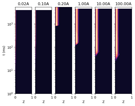
Next we simply show the profiles of temperature and hydroxyl mass fraction with the various rate parameters. We not only see the expected decrease in ignition delay with larger pre-exponential factor, but also that ignition does not occur at lower values as chain-branching is entirely overwhelmed by dissipation.

fig, axarray = plt.subplots(1, len(k1mult_list), sharex=True, sharey=True)

for k1mult in k1mult_list:
    sol = sol_dict[k1mult]
    axarray[sol[0]].contourf(sol[2], sol[1] * 1.e3, sol[3],
                             cmap=plt.get_cmap('magma'),
                             levels=np.linspace(300., max_temp, 20))
    axarray[sol[0]].set_title(f'{k1mult:.2f}A')
    axarray[sol[0]].set_xlim([0, 1])
    axarray[sol[0]].set_ylim([1.e0, max_time * 1.e3])
    axarray[sol[0]].set_yscale('log')
    axarray[sol[0]].set_xlabel('Z')

axarray[0].set_ylabel('t (ms)')
plt.show()

fig, axarray = plt.subplots(1, len(k1mult_list), sharex=True, sharey=True)

print('Mass fraction OH profiles')

for k1mult in k1mult_list:
    sol = sol_dict[k1mult]
    axarray[sol[0]].contourf(sol[2], sol[1] * 1.e3, sol[4],
                             cmap=plt.get_cmap('magma'))
    axarray[sol[0]].set_title(f'{k1mult:.2f}A')
    axarray[sol[0]].set_xlim([0, 1])
    axarray[sol[0]].set_ylim([1.e0, max_time * 1.e3])
    axarray[sol[0]].set_yscale('log')
    axarray[sol[0]].set_xlabel('Z')

axarray[0].set_ylabel('t (ms)')
plt.show()

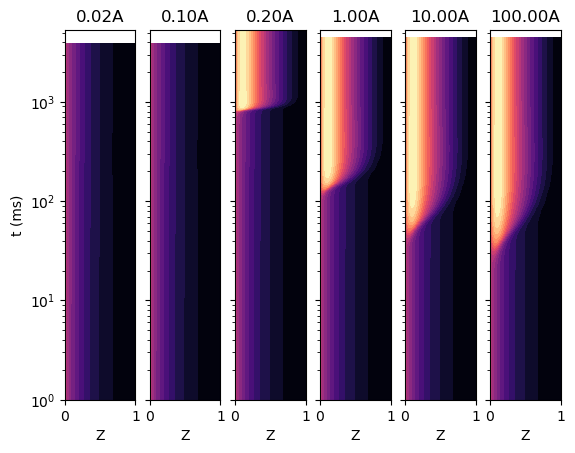
Mass fraction OH profiles