1.2.12. Transient Flamelet Example: Ignition and Advanced Time Integration
This demo is part of Spitfire, with licensing and copyright info here.
Highlights
Computing a transient ignition trajectory
Advanced time integration parameters
1.2.12.1. Introduction
In this demonstration we repeatedly compute the ignition trajectory of a hydrogen flamelet, using different time steppers, target errors for adaptive time step selection, and more.
from spitfire import ChemicalMechanismSpec, FlameletSpec, Flamelet
import cantera as ct
import matplotlib.pyplot as plt
import numpy as np
from time import perf_counter
Just as a reminder, here we build the chemical mechanism instace from a Cantera solution instead of simply providing the XML file and group name directly. Either works, but sometimes you might already have a Cantera solution available.
Following that, we build a preheated air stream and a fuel mixture of
Nitrogen and Hydrogen that gives a chosen stoichiometric mixture
fraction. These are sent to a FlameletSpec object for later.
sol = ct.Solution('h2-burke.yaml', 'h2-burke')
mech = ChemicalMechanismSpec.from_solution(sol)

Tair = 1200.
pressure = 101325.
zstoich = 0.1

air = mech.stream(stp_air=True)
air.TP = Tair, pressure
fuel = mech.mix_fuels_for_stoich_mixture_fraction(mech.stream('TPX', (Tair, pressure, 'H2:1')), mech.stream('TPX', (Tair, pressure, 'N2:1')), zstoich, air)
fuel.TP = 300., pressure

flamelet_specs = FlameletSpec(mech_spec=mech,
                              initial_condition='unreacted',
                              oxy_stream=air,
                              fuel_stream=fuel,
                              grid_points=34,
                              max_dissipation_rate=1.e3)
1.2.12.2. Baseline Ignition Trajectory
First, we’ll simply call integrate_to_steady without any parameters
to compute a flamelet ignition trajectory with the default time
integration settings.
ft = Flamelet(flamelet_specs)
output = ft.integrate_to_steady()
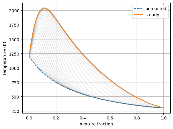
for i in range(0, output.time_values.size, 20):
plt.plot(output.mixture_fraction_values, output['temperature'][i, :], color='gray', alpha=0.2)
plt.plot(output.mixture_fraction_values, output['temperature'][0, :], '--', label='unreacted')
plt.plot(output.mixture_fraction_values, output['temperature'][-1, :], label='steady')
plt.grid()
plt.xlabel('mixture fraction')
plt.ylabel('temperature (K)')
plt.legend()
plt.show()
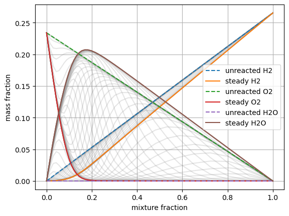
for i in range(0, output.time_values.size, 20):
plt.plot(output.mixture_fraction_values, output['mass fraction H2'][i, :], color='gray', alpha=0.2)
plt.plot(output.mixture_fraction_values, output['mass fraction O2'][i, :], color='gray', alpha=0.2)
plt.plot(output.mixture_fraction_values, output['mass fraction H2O'][i, :], color='gray', alpha=0.2)
plt.plot(output.mixture_fraction_values, output['mass fraction H2'][0, :], '--', label='unreacted H2')
plt.plot(output.mixture_fraction_values, output['mass fraction H2'][-1, :], label='steady H2')
plt.plot(output.mixture_fraction_values, output['mass fraction O2'][0, :], '--',label='unreacted O2')
plt.plot(output.mixture_fraction_values, output['mass fraction O2'][-1, :], label='steady O2')
plt.plot(output.mixture_fraction_values, output['mass fraction H2O'][0, :],'--', label='unreacted H2O')
plt.plot(output.mixture_fraction_values, output['mass fraction H2O'][-1, :], label='steady H2O')
plt.grid()
plt.xlabel('mixture fraction')
plt.ylabel('mass fraction')
plt.legend()
plt.show()
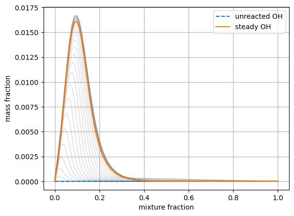
for i in range(0, output.time_values.size, 20):
plt.plot(output.mixture_fraction_values, output['mass fraction OH'][i, :], color='gray', alpha=0.2)
plt.plot(output.mixture_fraction_values, output['mass fraction OH'][0, :], '--', label='unreacted OH')
plt.plot(output.mixture_fraction_values, output['mass fraction OH'][-1, :], label='steady OH')
plt.grid()
plt.xlabel('mixture fraction')
plt.ylabel('mass fraction')
plt.legend()
plt.show()
1.2.12.3. Time Steppers and Target Error
Now we import some of Spitfire’s built-in time stepping methods. These
include BDF-1 (Backward Euler) and some implicit Runge-Kutta methods of
orders 3-5. The SimpleNewtonSolver is needed as the nonlinear solver
for the implicit time methods.
from spitfire import (SimpleNewtonSolver,
                      BackwardEulerS1P1Q1,
                      KennedyCarpenterS6P4Q3,
                      KvaernoS4P3Q2,
                      KennedyCarpenterS4P3Q2,
                      KennedyCarpenterS8P5Q4)
To run with a custom stepper, provide the stepper_type argument. A
related parameter in these adaptive steppers is the
transient_tolerance, which should be decreased to improve accuracy
through smaller time steps. This parameter relates to efficiency through
the order of the integration technique - for first-order (P1) Backward
Euler the relationship is linear and a ten times reduction in the
tolerance should roughly correspond to a ten times increase in run time.
For the P3, P4, and P5 methods, however, a factor of ten increase in run
time can enable a tolerance 1000, 10000, and 100000 times smaller,
respectively. This gives high-order methods a dramatic advantage in
solving to extreme accuracy, and in practice their better stability also
makes them faster at computing flamelet solutions without concern of
error.
Below we iterate over some combinations of methods and tolerances, followed by some results and discussion.
output_dict = dict()

for name, method, tol in [('BDF1', BackwardEulerS1P1Q1, 1e-7),
                          ('Kv-P3', KvaernoS4P3Q2, 1e-7),
                          ('KC-P3', KennedyCarpenterS4P3Q2, 1e-7),
                          ('KC-P4', KennedyCarpenterS6P4Q3, 1e-7),
                          ('KC-P5', KennedyCarpenterS8P5Q4, 1e-7),
                          ('BDF1', BackwardEulerS1P1Q1, 1e-8),
                          ('Kv-P3', KvaernoS4P3Q2, 1e-10),
                          ('KC-P3', KennedyCarpenterS4P3Q2, 1e-10),
                          ('KC-P4', KennedyCarpenterS6P4Q3, 1e-11),
                          ('KC-P5', KennedyCarpenterS8P5Q4, 1e-12)]:
    print(f'Running w/{name:5}, tolerance {tol:5.1e} ... ', end='')

    tic = perf_counter()
    ft = Flamelet(flamelet_specs)
    the_output = ft.integrate_to_steady(stepper_type=method, transient_tolerance=tol)
    dcput = perf_counter() - tic
    nsteps = the_output.time_values.size
    output_dict[(name, tol)] = (the_output, nsteps, dcput)

    print(f'done in {nsteps:5} time steps in {dcput:4.1f} s, mean cput/step of {dcput*1e3/nsteps:3.1f} ms')
Running w/BDF1 , tolerance 1.0e-07 ...
done in  5195 time steps in  6.6 s, mean cput/step of 1.3 ms
Running w/Kv-P3, tolerance 1.0e-07 ... done in   872 time steps in  2.9 s, mean cput/step of 3.3 ms
Running w/KC-P3, tolerance 1.0e-07 ... done in   396 time steps in  2.4 s, mean cput/step of 6.1 ms
Running w/KC-P4, tolerance 1.0e-07 ... done in   153 time steps in  1.2 s, mean cput/step of 8.1 ms
Running w/KC-P5, tolerance 1.0e-07 ... done in   112 time steps in  1.2 s, mean cput/step of 10.6 ms
Running w/BDF1 , tolerance 1.0e-08 ... done in 16227 time steps in 18.9 s, mean cput/step of 1.2 ms
Running w/Kv-P3, tolerance 1.0e-10 ... done in  8580 time steps in 13.0 s, mean cput/step of 1.5 ms
Running w/KC-P3, tolerance 1.0e-10 ... done in  3677 time steps in  7.6 s, mean cput/step of 2.1 ms
Running w/KC-P4, tolerance 1.0e-11 ... done in  1169 time steps in  4.9 s, mean cput/step of 4.2 ms
Running w/KC-P5, tolerance 1.0e-12 ... done in   774 time steps in  4.9 s, mean cput/step of 6.4 ms
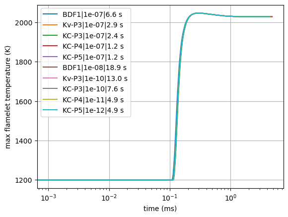
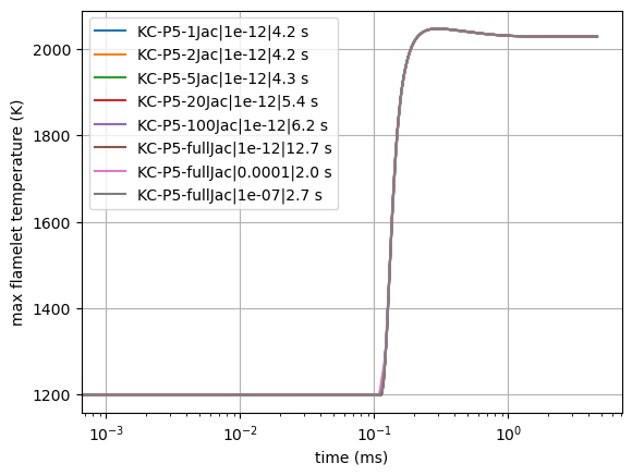
From the plot of maximum flamelet temperature, we can see that the ignition delay time seems similar across all of the methods and target errors. This is a typical observation in transient flamelet models - a solution that stays stable will usually be sufficiently accurate (in terms of time integration error - other errors are still relevant).
Some interesting observations can be made from the efficiency numbers.
Higher-order methods are the fastest for a given tolerance, both for high, stability-limited values and lower values meant for accurate simulations.
Higher-order methods require more CPU time per step but take fewer steps.
Higher-order methods are significantly faster at computing solutions with lower tolerances
Decreasing the tolerance decreases the CPU time per step
The first three conclusions are not surprising, but the fourth one is confusing at first. The reason the CPU time per step decreases with tolerance is that Spitfire, similarly to other advanced ODE solvers, not only adaptively changes the time step size but also adaptively evaluates/factorizes the Jacobian matrix. Expensive calculations with the Jacobian are kept to a minimum, and can be minimized further when the error tolerance is lower. This is because smaller time steps fail less frequently and give smoother behavior when nonlinear transients appear suddenly. Jacobian reuse is why KC-P4 (Spitfire’s default stepper) is nearly twice as fast per time step at the lower tolerance (\(10^{-11}\)) than the higher one - however, the increase in time step count does still increase the runtime.
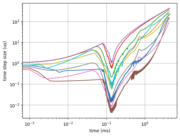
The second plot below shows the time step size history for each solver. Observe especially how BDF-1 with tolerance of \(10^{-8}\) requires the smallest step size, compared to the higher-order methods with much lower tolerances. The fifth-order method (KC-P5) is always taking a time step at least an order of magnitude larger, even at a tolerance of \(10^{-12}\).
for name, transient_tol in output_dict:
    output, nsteps, dcput = output_dict[(name, transient_tol)]
    plt.semilogx(output.time_values * 1.e3, np.max(output['temperature'], axis=1), label=f'{name}|{transient_tol}|{dcput:.1f} s')
plt.grid()
plt.xlabel('time (ms)')
plt.ylabel('max flamelet temperature (K)')
plt.legend()
plt.show()

for name, transient_tol in output_dict:
    output, nsteps, dcput = output_dict[(name, transient_tol)]
    t = output.time_values
    dt = t[1:] - t[:-1]
    plt.loglog(t[:-1] * 1.e3, dt * 1.e6, label=f'{name}/{transient_tol:.1e} | {dcput:.1f} s')
plt.grid()
plt.xlabel('time (ms)')
plt.ylabel('time step size (us)')
plt.show()
1.2.12.4. Jacobian/Preconditioner Reuse
We can roughly control the degree of Jacobian/preconditioner reuse with
the maximum_steps_per_jacobian argument to integrate_to_steady,
which maps to the linear_setup_rate argument in Spitfire’s
odesolve method. Setting this argument to 1 means we always
re-evaluate the Jacobian on every time step. Setting it to 20, for
instance, simply means that a maximum of 20 steps can occur between
re-evaluation/factorization. The default setting in
integrate_to_steady is 10, and while it is tempting to increase it
further, this can negatively impact stability and force smaller time
steps during nonlinear transients.
Other parameters such as time_step_increase_factor_to_force_jacobian
and time_step_decrease_factor_to_force_jacobian to odesolve can
be used to control Jacobian/preconditioner reuse.
Also we can build the nonlinear solver differently. The
SimpleNewtonSolver class can be built with the
evaluate_jacobian_every_iter argument set to True. This can be
provided through integrate_to_steady with the
extra_nlsolver_args argument (takes a dictionary of keyword
arguments to be passed to the nonlinear solver construction). This goes
a step further than maximum_steps_per_jacobian=1, never reusing the
Jacobian matrix even between nonlinear solver iterations. This improves
stability quite a bit, and reduces nonlinear iteration count, but for
larger mechanisms (more species) this is extremely costly. For hydrogen,
however, it’s still pretty cheap and works out well in the end.
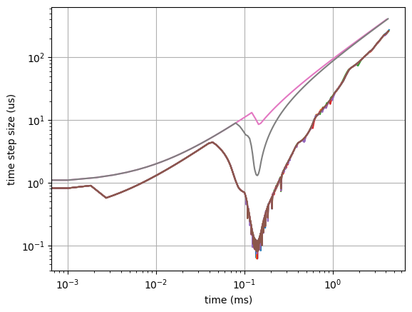
Below we run the fifth-order method with different values of
maximum_steps_per_jacobian and then with the Jacobian re-evaluated
at every Newton iteration. This enables us to get past the
\(10^{-7}\) tolerance limit imposed by stability on the lagged
Jacobian runs, leading to very fast solutions. I’ll repeat it though -
this option is much slower (take a look at the CPU time per step) and is
impractical for larger mechanisms where the Jacobian
evaluation/factorization is the dominant cost.
for name, method, tol, mspj, nlsa in [('KC-P5-1Jac', KennedyCarpenterS8P5Q4, 1e-12, 1, dict()),
                                      ('KC-P5-2Jac', KennedyCarpenterS8P5Q4, 1e-12, 2, dict()),
                                      ('KC-P5-5Jac', KennedyCarpenterS8P5Q4, 1e-12, 5, dict()),
                                      ('KC-P5-20Jac', KennedyCarpenterS8P5Q4, 1e-12, 20, dict()),
                                      ('KC-P5-100Jac', KennedyCarpenterS8P5Q4, 1e-12, 100, dict()),
                                      ('KC-P5-fullJac', KennedyCarpenterS8P5Q4, 1e-12, 1, {'evaluate_jacobian_every_iter': True}),]:
    print(f'Running w/{name:15}, tolerance {tol:5.1e} ... ', end='')
    tic = perf_counter()
    ft = Flamelet(flamelet_specs)
    the_output = ft.integrate_to_steady(stepper_type=method,
                                        transient_tolerance=tol,
                                        maximum_steps_per_jacobian=mspj,
                                        extra_nlsolver_args=nlsa)
    dcput = perf_counter() - tic
    nsteps = the_output.time_values.size
    output_dict[(name, tol)] = (the_output, nsteps, dcput)
    print(f'done in {nsteps:5} time steps in {dcput:4.1f} s, mean cput/step of {dcput*1e3/nsteps:3.1f} ms')
Running w/KC-P5-1Jac , tolerance 1.0e-12 ...
done in   777 time steps in  4.2 s, mean cput/step of 5.4 ms
Running w/KC-P5-2Jac     , tolerance 1.0e-12 ... done in   774 time steps in  4.2 s, mean cput/step of 5.5 ms
Running w/KC-P5-5Jac     , tolerance 1.0e-12 ... done in   769 time steps in  4.3 s, mean cput/step of 5.6 ms
Running w/KC-P5-20Jac    , tolerance 1.0e-12 ... done in   779 time steps in  5.4 s, mean cput/step of 7.0 ms
Running w/KC-P5-100Jac   , tolerance 1.0e-12 ... done in   779 time steps in  6.2 s, mean cput/step of 8.0 ms
Running w/KC-P5-fullJac  , tolerance 1.0e-12 ... done in   773 time steps in 12.7 s, mean cput/step of 16.5 ms
for name, method, tol, mspj, nlsa in [('KC-P5-fullJac', KennedyCarpenterS8P5Q4, 1e-4, 1, {'evaluate_jacobian_every_iter': True}),
                                      ('KC-P5-fullJac', KennedyCarpenterS8P5Q4, 1e-7, 1, {'evaluate_jacobian_every_iter': True})]:
    print(f'Running w/{name:15}, tolerance {tol:5.1e} ... ', end='')
    tic = perf_counter()
    ft = Flamelet(flamelet_specs)
    the_output = ft.integrate_to_steady(stepper_type=method,
                                        transient_tolerance=tol,
                                        maximum_steps_per_jacobian=mspj,
                                        extra_nlsolver_args=nlsa)
    dcput = perf_counter() - tic
    nsteps = the_output.time_values.size
    output_dict[(name, tol)] = (the_output, nsteps, dcput)
    print(f'done in {nsteps:5} time steps in {dcput:4.1f} s, mean cput/step of {dcput*1e3/nsteps:3.1f} ms')
Running w/KC-P5-fullJac  , tolerance 1.0e-04 ... done in    72 time steps in  2.0 s, mean cput/step of 27.6 ms
Running w/KC-P5-fullJac  , tolerance 1.0e-07 ... done in   106 time steps in  2.7 s, mean cput/step of 25.2 ms
for name, transient_tol in output_dict:
    if 'KC-P5' in name and 'Jac' in name:
        output, nsteps, dcput = output_dict[(name, transient_tol)]
        plt.semilogx(output.time_values * 1.e3, np.max(output['temperature'], axis=1), label=f'{name}|{transient_tol}|{dcput:.1f} s')
plt.grid()
plt.xlabel('time (ms)')
plt.ylabel('max flamelet temperature (K)')
plt.legend()
plt.show()

for name, transient_tol in output_dict:
    if 'KC-P5' in name and 'Jac' in name:
        output, nsteps, dcput = output_dict[(name, transient_tol)]
        t = output.time_values
        dt = t[1:] - t[:-1]
        plt.loglog(t[:-1] * 1.e3, dt * 1.e6, label=f'{name}/{transient_tol:.1e} | {dcput:.1f} s')
plt.grid()
plt.xlabel('time (ms)')
plt.ylabel('time step size (us)')
plt.show()
1.2.12.5. Conclusions
In this notebook we’ve solved a transient flamelet ignition problem with a number of different time integration settings. There’s more that can be modified but these are the major options. We’ve shown the merit of high-order methods provided by Spitfire and shown some results regarding Jacobian/preconditioner reuse.