1. Reaction Models
1.1. Background
The following sections detail the backround and some of the math behind Spitfire’s reaction modeling capabilities. We present the background of non-premixed flamelet models and then of simpler homogeneous reactor systems, and supported reaction rate laws and thermodynamic property models.
1.1.1. Flamelet Modeling Background
Mixture Fraction Models
The basic starting point for modeling reacting flows is direct numerical simulation (DNS), an approach wherein governing equations for mass, momentum, energy, and species transport are solved on fine grids with small time steps to simply resolve every scale present in the problem. The range of time and length scales as well as state space dimensionality make DNS impossible for engineering analysis of turbulent flows with current computing capabilities. This motivates turbulence models that require closure of thermochemical state evolution. For non-premixed flames an effective approach is RANS or LES with mixture fraction modeling. Here we describe mixture fraction models for low-Mach combustion applications, particularly large pool fires, and we avoid getting into the details of RANS vs LES models. See Domino et al. [DHKH20201] for a more detailed overview, particularly focused on capabilities and applications at Sandia National Laboratories (SNL).
Stefan P. Domino and John C. Hewson and Robert C. Knaus and Michael A Hansen, Predicting large-scale pool fire dynamics using an unsteady flamelet- and large-eddy simulation-based model suite, Physics of Fluids, Volume 33, 2021
In mixture fraction models the standard set of filtered continuity and momentum equations are solved along with any equations needed by the turbulence model (e.g., a \(k-\varepsilon\) model requires two additional equations). For large, sooting fires radiation plays a significant role and must be modeled, typically through a discrete ordinates approach. The remaining ingredient to a mixture fraction model is the evolution of the thermochemical state. Solving transport equations for a detailed set of chemical species is impractical due to the large numbers of species and reactions and the difficulty of accurately predicting subgrid fuel consumption. Mixture fraction models simultaneously address the issues of state space dimensionality and turbulent closure, separating the small-scale resolution of detailed chemical reactions from the large-scale evolution of a fire.
All mixture fraction models solve at least one additional transport equation for the mixture fraction, a conserved scalar that measures fuel/air mixing. RANS models include at least one more equation for the subgrid variance of the mixture fraction (the scalar variance), while LES models typically presume a gradient closure to measure subgrid variance.
Equilibrium & Burke-Schumann Models
Presuming that combustion chemistry happens infinitely fast leads to equilibrium or Burke-Schumann models, wherein the mixture fraction and its variance completely describe the thermochemical state. These models are distinguished by their treatment of chemistry - equilibrium corresponds to minimization of the Gibbs free energy while Burke-Schumann presumes idealized combustion. For a laminar flame (the limit of zero subgrid scalar variance) this means the temperature and mass fractions are known from the local mixture fraction alone. This is an extreme assumption on scale separation - presuming that chemistry responds so fast that it may be completely decoupled from the fluid dynamics.
Strained Laminar Flamelet Models
Improved mixture fraction models incorporate the effects of local fluid strain on combustion chemistry. A useful measure of the strain rate is the scalar dissipation rate, \(\chi=2D\|\nabla\mathcal{Z}\|^2\), where \(D\) is the diffusivity of the mixture fraction (typically near the thermal diffusivity). In these models gas state variables and properties are known from the mixture fraction, scalar variance, and scalar dissipation rate, with the dissipation rate computed in a variety of ways in LES/RANS approaches. At high enough strain rates flames can locally extinguish although this is not typically included in these models. While this type of model is still assuming scale separation, the effects of finite rate chemistry are included through a diffusive-reactive balance described by the flamelet equations parameterized by the scalar dissipation rate. This is referred to as a strained laminar flamelet model, or SLFM. An essential assumption to SLFM is that to solve the flamelet equations of an SLFM method one must presume a correlation of the scalar dissipation rate and mixture fraction, \(\chi(\mathcal{Z})\). Spitfire’s preliminary aim related to the solution of the reaction-diffusion equations needed to build SLFM chemistry libraries.
Non-adiabatic Flamelet Models
An additional advancement of mixture fraction models is necessary for application to large-scale sooting fires: non-adiabaticity of the flame. Radiative losses to soot and exposed surfaces removes the correlation of mixture fraction and enthalpy that holds for adiabatic flows. In non-adiabatic mixture fraction models the fire model must determine the extent of departure from adiabatic conditions, and the flamelet model must account for the effect of this departure on small-scale combustion chemistry. Similarly to the dissipation rate of SLFM models, the effect of radiation on the flamelet equations must be modeled in mixture fraction space. Alternatively one may alter boundary stream enthalpies. Equation modifications typically take the form of temperature-dependent source terms to model radiative quenching/extinction, although superadiabaticity in extremely large fires may be important as well. Two approaches to equation modification are supported in Spitfire and will be presented in detail in a following section. Non-adiabatic equilibrium and Burke-Schumann flamelets may also be constructed with Spitfire, and this will also be presented later.
Turbulence Modeling: Presumed PDF Tabulation
An important step for RANS/LES calculations is the closure problem: modeling the effects of subgrid (unresolved) phenomena on resolved scales. With presumed PDF models, one can view the various flamelet models discussed above as “chemistry models” or “reaction models” and the problem of subgrid closure requires a follow-on “mixing model.” Simple presumed PDF models require convolution of tabulated flamelet solutions over the mixture fraction dimension for a range of scalar variances. This is discussed in two demonstrations, Tabulation API Example: Presumed PDF SLFM Tables and Custom Presumed PDF: log-mean PDF of the scalar dissipation rate.
Soot Modeling
One final step to the solution of sooting fires is the modeling of soot, which is often done with a moment method or sectional method. An efficient, semi-empirical method appropriate for engineering analysis is a two-equation soot model where transport equations for the number and mass density of soot particles are solved. Such a model requires source terms for soot formation/destruction based on the local thermochemical state. Physical processes such as particle coagulation are resolved by the fire model, but chemical processes such as gas phase precursor formulation, nucleation, condensation, surface growth and oxidation depend on the flamelet model for the chemistry. Soot moments are solved in the fire model because soot particles evolve relatively slowly and their effective diffusion rates are low compared to gas species. It is inappropriate to presume that soot particles follow the same diffusive-reactive equilibrium as gas species, and so we compute coefficients, or propensity terms, for soot growth/oxidation/nucleation/etc. in a flamelet library. More details on tabulating these coefficients can be found in Soot Models
Tabulation
The various flamelet formulations described above can be prepared in advance and tabulated so that equilibrium/flamelet solutions do not need to be computed in situ during a simulation. Spitfire currently provides several layers of abstraction for building flamelet libraries in the form of structured interpolation tables, and is actively involved in research into unstructured tabulation approaches (e.g., neural networks that do not employ tensor product interpolation). Direct support is available for tables used at Sandia National Laboratories for hydrocarbon pool fire models, although Spitfire is designed to allow advanced users to tabulate libraries for their own formulations.
1.1.2. Governing Equations for Non-premixed Flamelets
Spitfire’s flamelet and tabulation capabilities support generalized flamelet models for RANS/LES of hydrocarbon pool fires in the non-premixed combustion regime. While direct support is provided for sooting hydrocarbon fires, Spitfire leverages a modular, extensible stack from thermochemistry evaluator, numerical methods, solvers, and tabulation techniques. In this section we detail the governing equations solved by Spitfire for equilibrium, strained steady/transient, adiabatic/non-adiabatic flamelets. All of these equations are defined with the mixture fraction coordinate. These equations can be derived in a variety of ways, either through local coordinate transformations along the isosurfaces of the mixture fraction or by transforming species transport equations to follow a general Lagrangian coordinate frame. In both cases, time and length scale separation arguments lead to one-dimensional equilibrium/strained/non-adiabatic flamelet models of flows with two inlets.
Strained Flamelet Models
The thermochemical state is described with the mass fractions \(Y_i\) and temperature \(T\). These are described by the mixture fraction \(\mathcal{Z}\) and other parameters, and in transient flamelets we consider evolution in a Lagrangian time \(t\). Equations (1.1) and (1.2) describe adiabatic flamelets, which balance molecular mixing (with strength proportional the scalar dissipation rate \(\chi\)) with species production/consumption and heat release through chemical reactions. These equations include variable heat capacity effects and the full form of the heat flux including the diffusive enthalpy terms. They do not account for differential diffusion and are based on a unity Lewis number and mass fraction form of the species diffusive fluxes. Generalizations of the diffusive flux models have been derived and are planned for a future version of Spitfire. The variable heat capacity term and enthalpy flux terms are optional in Spitfire, but are included by default as they are very important for modeling non-adiabatic flows with strong coupling to radiative losses. The steady version of this equation set is derived by simply removing the time derivative term.
These equations are supplemented by Dirichlet boundary conditions defined by the oxidizer and fuel states,
The dissipation rate \(\chi\) can be a constant or depend on the mixture fraction. Spitfire provides the common form due to Peters:
Non-Adiabatic Strained Flamelet Models
Spitfire also supports non-adiabatic flamelet models. Non-adiabaticity modifies the temperature equation through the inclusion of source terms,
The convection and radiation coefficients and reference temperatures are allowed to vary over the mixture fraction. Further, the heat loss terms can be scaled to facilitate simulation of strong radiative quenching in large sooting fires,
where \(\mathcal{Z}_{\mathrm{st}}\) is the stoichiometric mixture fraction. The preferred model supported in Spitfire for hydrocarbon pool fires is to use a convective/linear form of the heat loss with \(h'\) to \(10^6-10^7\), which rapidly drives hydrocarbon flamelets to extinction, covering a wide range of the heat loss space broadly throughout the mixture fraction. Spitfire also provides a quasi-steady continuation approach for non-adiabatic SLFM models.
Equilibrium Models
The previous section provides unsteady flamelet equations for adiabatic and non-adiabatic flames. Steady flamelet models for SLFM tabulation are obtained by neglecting the time derivative terms. Equilibrium models are derived by neglecting the dissipation terms as well. Here the temperature equation can be replaced with a constant total enthalpy equation (\(h_t=0\)), which is a more basic expression than the temperature equations above. Minimizing the Gibbs free energy at each grid point in \(\mathcal{Z}\) then produces the desired equilibrium solution. Spitfire does not provide an equilibrium solver, instead using the well-proven capability of Cantera for equilibrium calculations.
Burke-Schumann Models
Burke-Schumann flamelet models are based on a presumption of infinitely fast and idealized combustion, wherein fuel and oxygen are consumed to produce water and carbon dioxide products, to the extent afforded by local stoichiometry. At the stoichiometric mixture fraction this results in complete combustion. The enthalpy of the mixture is kept at its linear value between the fuel/oxidizer streams, and mass fractions are computed with the ideal combustion assumption. The temperature is then computed given the enthalpy and composition, often resulting in sharp peaks at \(\mathcal{Z}_{\mathrm{st}}\) and nearly linear profiles on the lean and rich sides.
Non-Adiabatic Equilibrium and Burke-Schumann Models
The non-strained flamelet models can be augmented to account for non-adiabaticity in a number of ways. In Spitfire we implement a fairly simple formulation. A piecewise linear function of mixture fraction, zero at the boundaries and unity at \(\mathcal{Z}_{\mathrm{st}}\), is multiplied by a (negative) stoichiometric enthalpy defect parameter to offset the enthalpy of the mixture, and then one simply recomputes equilibrium/Burke-Schumann profiles with this perturbed enthalpy. This is performed for enthalpies spanning the nonreacted enthalpy and the enthalpy of a completely extinguished mixture to model the full extent of radiative quenching/extinction.
An intriguing and untested alternative more consistent with the SLFM approach is to introduce a temperature source term. This results in a collection of transient homogeneous reactor problems, which could be solved in tandem and tabulated as if they were flamelet equations with zero strain. This may lead to a very different quenching behavior than the imposed enthalpy defect profiles, although this is likely not worth pursuing simply due to the limitations of equilibrium/Burke-Schumann models.
1.1.3. Tabulation Approach for Turbulent Pool Fires
1.1.3.1. The FlameletSpec Class
The first step of building flamelet libraries is to specify the thermochemistry, mixture fraction grid, boundary streams, and flamelet equation set.
Spitfire provides the FlameletSpec class to contain this information, which is detailed below.
FlameletSpec instances can be created by specifying these parameters directly or
by providing a one-dimensional slice of a Library object with a mech_spec object as an extra_attribute.
The library option is extremely convenient when building multidimensional flamelet libraries.
- thermochemistry:
mech_spec: aSpitfire.ChemicalMechanismSpecobject representing gas thermochemistry (species thermal data, transport data, reaction rate data)initial_condition: a string (see Building Adiabatic Non-Strained Libraries) or numpy.ndarray for the interior state variables (a ravel`ed grid with temperature and :math:`n-1 mass fractions for \(n_{\mathcal{Z}}-2\) grid points)
- discretization of the mixture fraction:
grid: directly specify a set of grid point locations, overriding any other parametersgrid_points: specify the number of grid pointsgrid_type: specify to use a “clustered” grid or a “uniform” gridgrid_cluster_point: mixture fraction value around which a “clustered” grid refines the mesh, can be “stoichiometric” to cluster around \(\mathcal{Z}_{\mathrm{st}}\)grid_cluster_intensity: how tightly a “clustered” grid reduces the grid spacing around its cluster point
- boundary streams:
oxy_stream: CanteraQuantityorSolutioninstance for the oxidizer (\(\mathcal{Z}=0\))fuel_stream: CanteraQuantityorSolutioninstance for the fuel (\(\mathcal{Z}=1\))
- equation terms:
include_enthalpy_flux: whether or not to include the enthalpy diffusion term, see (1.2)include_variable_cp: whether or not to include the variable heat capacity term (heat capacities are always modeled as specified in the chemical mechanism), see (1.2)- heat loss formulation
heat_transfer: whether the flamelets are “adiabatic” or “non-adiabatic”convection_temperature: directly specify a constant or \(\mathcal{Z}\)-dependent value for \(T_\infty\)radiation_temperature: directly specify a constant or \(\mathcal{Z}\)-dependent value for \(T_{\mathrm{surf}}\)convection_coefficient: directly specify a constant or \(\mathcal{Z}\)-dependent value for \(h\)radiative_emissivity: directly specify a constant or \(\mathcal{Z}\)-dependent value for \(\varepsilon\)scale_heat_loss_by_temp_range: whether or not to include the \(T_\max\) terms in (1.6)scale_convection_by_dissipation: whether or not to multiply both heat loss terms by \(\chi_\max\) in (1.6)use_linear_ref_temp_profile: specifies a linear temperature profile for \(T_\infty\) and \(T_{\mathrm{surf}}\) based on the stream temperatures
- dissipation rate formulation
dissipation_rate: option to specify the dissipation rate evaluated on the mixture fraction grid, ignores all other dissipation rate optionsdissipation_rate_form: whether to use a “Peters” or a constant dissipation rate form, based on the given maximum or stoichiometric valuesmax_dissipation_rate: if using the “Peters” or constant dissipation rate, calibrate the curve to hit this maximum valuestoich_dissipation_rate: if using the “Peters” or constant dissipation rate, calibrate the curve to hit this value at the stoichiometric mixture fraction
1.1.3.2. The Flamelet Class
After building an instance of the FlameletSpec class,
we build a Flamelet instance.
The Flamelet class provides basic interfaces for the flamelet equations,
namely initializing to equilibrium and Burke-Schumann solutions (see Building Adiabatic Non-Strained Libraries)
and computing steady/transient solutions.
To compute steady solutions, the Flamelet class provides the compute_steady_state method,
which will use the initial condition of the flamelet as a first guess and attempt to compute the steady flamelet solution with a variety of solvers.
Constructing SLFM tables can often be done by chaining together calls to compute_steady_state while traversing a parameter space.
For transient flamelets, the integrate method wraps a call to Spitfire’s odesolve function,
and methods like integrate_to_steady, integrate_to_time, integrate_to_steady_after_ignition, integrate_for_heat_loss, and compute_ignition_delay
further provide simpler interfaces around integrate.
Residuals and Jacobian matrices are computed with code in Spitfire’s C++ engine, Griffon,
and abstract numerical algorithms like Newton’s method and time integration are coded directly in Python.
A specialized version of Newton’s method exists for flamelets as well as a novel pseudotransient continuation approach (CITE MJ SIAM/CTM).
The Flamelet class provides the rhs and jac methods so a user may directly write their own solvers or use external time integrators.
jac provides the Jacobian in a form suitable for a particular linear solver,
and the jac_csc method converts this to a SciPy CSC format.
Spitfire can be made to use the SuperLU solver provided through SciPy, but Spitfire’s built-in solver is signficantly faster
because it is explicitly designed for the “block-tridiagonal-diagonal-offdiagonal matrices” we build for flamelets.
1.1.3.3. Building Adiabatic Non-Strained Libraries
Adiabatic, non-strained flamelet libraries are the simplest to construct.
Nonreacting, equilibrium, and Burke-Schumann flamelets can be obtained simply by initializing a Flamelet instance
with the appropriate initial_condition argument.
Flamelets may also be initialized to linear temperature and mass fractions through the FlameletSpec directly,
as an alternative to the nonreacting flamelets with linear enthalpy and mass fractions.
Several wrapper methods, termed “library builder” methods, are provided for convenience:
- build_unreacted_library: FlameletSpec(..., initial_condition='unreacted', ...)
- build_adiabatic_eq_library: FlameletSpec(..., initial_condition='equilibrium', ...)
- build_adiabatic_bs_library: FlameletSpec(..., initial_condition='Burke-Schumann', ...)
- no build_*_library method for extinguished states, use FlameletSpec(..., initial_condition='linear-TY', ...)
The build_*_library methods above are quite simple,
copying the provided FlameletSpec instance,
setting the initial_condition,
creating a Flamelet instance and then returning the desired Library.
For instance, a simple implementation of the equilibrium library is shown here:
def build_adiabatic_eq_library(flamelet_specs, verbose=True):
    # 1) copy flamelet specs, make FlameletSpecs if a dictionary is provided
    # 2) set the initial condition
    # 3) instantiate a ``Flamelet``
    # 4) return a ``Library`` object

    fs = FlameletSpec(**flamelet_specs) if isinstance(flamelet_specs, dict) else copy.copy(flamelet_specs)
    fs.initial_condition = 'equilibrium'
    flamelet = Flamelet(fs)
    return flamelet.make_library_from_interior_state(flamelet.initial_interior_state)
1.1.3.4. Building Adiabatic SLFM Libraries
To build adiabatic SLFM libraries we will Spitfire’s Flamelet.compute_steady_state() method along with one of the initialization approaches (Building Adiabatic Non-Strained Libraries).
This method is demonstrated along with transient flamelets and more by the Introduction to Flamelet Models & Spitfire demonstration.
The basic SLFM library is composed by computing a steady flamelet solution for low values of the scalar dissipation rate,
and then computing steady solutions for increasing \(\chi\) until reaching a specified value or when extinction occurs.
The build_adiabatic_slfm_library method manages this simple parameter continuation problem.
Default behavior is to initialize to the equilibrium flamelet first, and then directly solve for a list of specified maximum/stoichiometric dissipation rates.
Advanced users can fairly easily compose controller-type continuation approaches for more accurate (and possibly faster) tabulation,
and generalization of these techniques has long been on Spitfire’s to-do list.
The Tabulation API Example: Adiabatic Flamelet Models,
Tabulation API Example: Methane Shear Layer,
and Custom Tabulation Example: 4D Coal Combustion Model
pages demonstrate the use of build_adiabatic_slfm_library and Flamelet.compute_steady_state()
to generate several steady flamelet libraries.
The Custom Tabulation Example: 4D Coal Combustion Model demonstration showcases a four-dimensional
steady flamelet library with flame strain, heat loss, and variable fuel composition relevant to multiphase combustion.
1.1.3.5. Building Non-Adiabatic Non-Strained Libraries
To build nonadiabatic variants of the non-strained libraries, Spitfire employs a straightforward approach used at SNL. The initial adiabatic libraries are created as described above, and then a range of stoichiometric enthalpy defect values is traversed, recomputing equilibrium composition and temperature, or just the temperature for Burke-Schumann models, for each enthalpy profile. The build_nonadiabatic_defect_eq_library and build_nonadiabatic_defect_bs_library methods that execute this procedure do not leverage the Flamelet class very much beyond initialization. These tables could be built more easily if we improved Flamelet to allow enthalpy-based initialization (instead of temperature). Examples of non-adiabatic, non-strained flamelet libraries may be found in the Tabulation API Example: Nonadiabatic Flamelet Models demonstration.
1.1.3.6. Building Non-Adiabatic SLFM Libraries
Spitfire provides build_*_library methods for two approaches to building non-adiabatic strained laminar flamelet libraries. Each of these approaches builds a Library object with mixture fraction, dissipation rate, and stoichiometric enthalpy defect dimensions. At the moment neither of these capabilities can model super-adiabatic flamelets (e.g., positive “heat loss”).
build_nonadiabatic_defect_transient_slfm_library: transient quenching to a full enthalpy defect range, more uniform \(T(\mathcal{Z})\) profiles near extinction
build_nonadiabatic_defect_steady_slfm_library: quasi-steady heat loss, often does not extinguishe the mixture or reach very large enthalpy defect values
The transient version of heat loss is used at SNL to model large-scale sooting pool fires and has been carefully designed to cover a wide range of enthalpy defects (full radiative quenching) with broad heat loss profiles in mixture fraction. It relies on running what is ultimately an unstable calculation, solving (1.6) with all of the “corrections” applied to the convective heating term (the \(T^4\) term is not used despite the apparent relationship to radiative quenching) until the temperature is dropped to within 5% of the linear profile between the two streams. This is typically run with the convective heating coefficient at \(10^7\) to drive extreme heat loss. The integrate_for_heat_loss method on the Flamelet class is used to drive this transient calculation, and often several runs are attempted by Spitfire with lower and lower values of the time integration tolerance (increasing how conservatively we run adaptive time stepping). This is performed for each steady solution in an adiabatic SLFM table, and extension of the enthalpy defect for each dissipation rate can be run in parallel.
The quasi-steady version of heat loss uses the compute_steady_state method to perform continuation in the convective heat loss parameter. This is much more similar to typical SLFM tabulation approaches, but it typically does not result in as large of enthalpy defect ranges.
In both versions of the enthalpy defect extension, results are interpolated onto a grid of the stoichiometric enthalpy defect. This step introduces a slight amount of error but is necessary to allow structured (tensor product) interpolation in the downstream CFD code. Examples of these and non-strained variants may be found in the Tabulation API Example: Nonadiabatic Flamelet Models demonstration.
For some additional demonstrations of transient flamelet libraries, the Introduction to Flamelet Models & Spitfire demonstration shows a transient adiabatic flamelet model of extinction, and the Transient Flamelet Example: Ignition and Advanced Time Integration example show transient flamelet ignition calculations with a variety of high-order time integrators.
1.1.4. Governing Equations for Homogeneous Reactors
Homogeneous, or ‘zero-dimensional,’ reactor models represent well-mixed combustion systems wherein there are no spatial gradients in any quantity describing the chemical mixture. In such a system the temperature \(T\), pressure \(p\), and composition, expressed by the mass fractions \(\{Y_i\}\), are all homogeneous and a reactor may be modeled as a point in space whose properties vary only in time, \(t\). Zero-dimensional systems are idealizations of very complex systems but have their place in the modeling of combustion processes. In a lab setting this idealization can be approached with jet-stirred reactors (JSR, also commonly referred to as a continuous stirred tank reactor (CSTR), perfectly stirred reactor (PSR), and Longwell reactor) and rapid compression machines (RCM). A JSR is a continuous stirred tank reactor to which reactants are fed and mixed rapidly through several opposed jets. A JSR unit coupled with downstream gas chromatography and mass spectrometry can be used to quantify the composition of the chemical mixture as reaction proceeds. Detailed models of combustion kinetics are developed through comparison with experimental data from such systems. The rapid computational solution of kinetic models for simple, zero-dimensional reactors is of great fundamental importance to combustion modeling.
In Spitfire we model mixtures of ideal gases in twelve types of reactors distinguished by their configuration, heat transfer, and mass transfer. We use configuration to distinguish isochoric, or constant-volume, reactors from isobaric, or constant-pressure, ones. Mass transfer refers to a closed, or batch, reactor or an open reactor with mass flow at specified mean residence time. Three types of heat transfer are available:
adiabatic: a reactor with insulated walls that allow no heat transfer with the surroundings
isothermal: a reactor whose temperature is held exactly constant for all time
diathermal: a reactor whose walls allow a finite rate of heat transfer by radiative heat transfer to a nearby surface and convective heat transfer to a fluid flowing around the reactor
Below we detail the equations governing isochoric and isobaric reactors with any pair of models for mass and transfer. In all cases, the gas is modeled as a mixture of thermally perfect gases. The ideal gas law applies to each species and the bulk mixture.
where the mixture specific gas constant, \(R_\mathrm{mix}\), is the universal molar gas constant divided by the mixture molar mass,
where \(M_i\) is the molar mass of species \(i\) in a mixture with \(n\) distinct species. Additionally, the mass fractions, of which only \(n-1\) are independent (and only \(n-1\) are solved for in Spitfire), are related by
1.1.5. Isochoric Reactors
Figure Fig. 1.1 diagrams an open, constant-volume reactor with diathermal walls. The reactor has volume \(V\) and surface area \(A\). Convective heat transfer is described by a fluid temperature \(T_\infty\) and convective heat transfer coefficient \(h\). Radiative heat transfer is determined by the temperature of the surface, \(T_\mathrm{surf}\), and effective emissivity, \(\varepsilon\). Finally, for an isochoric reactor, mass transfer is specified by the residence time \(\tau\), based on volumetric flow rate, and inflowing state with temperature \(T_\mathrm{in}\), density \(\rho_\mathrm{in}\), and mass fractions \(\{Y_{i,\mathrm{in}}\}\).
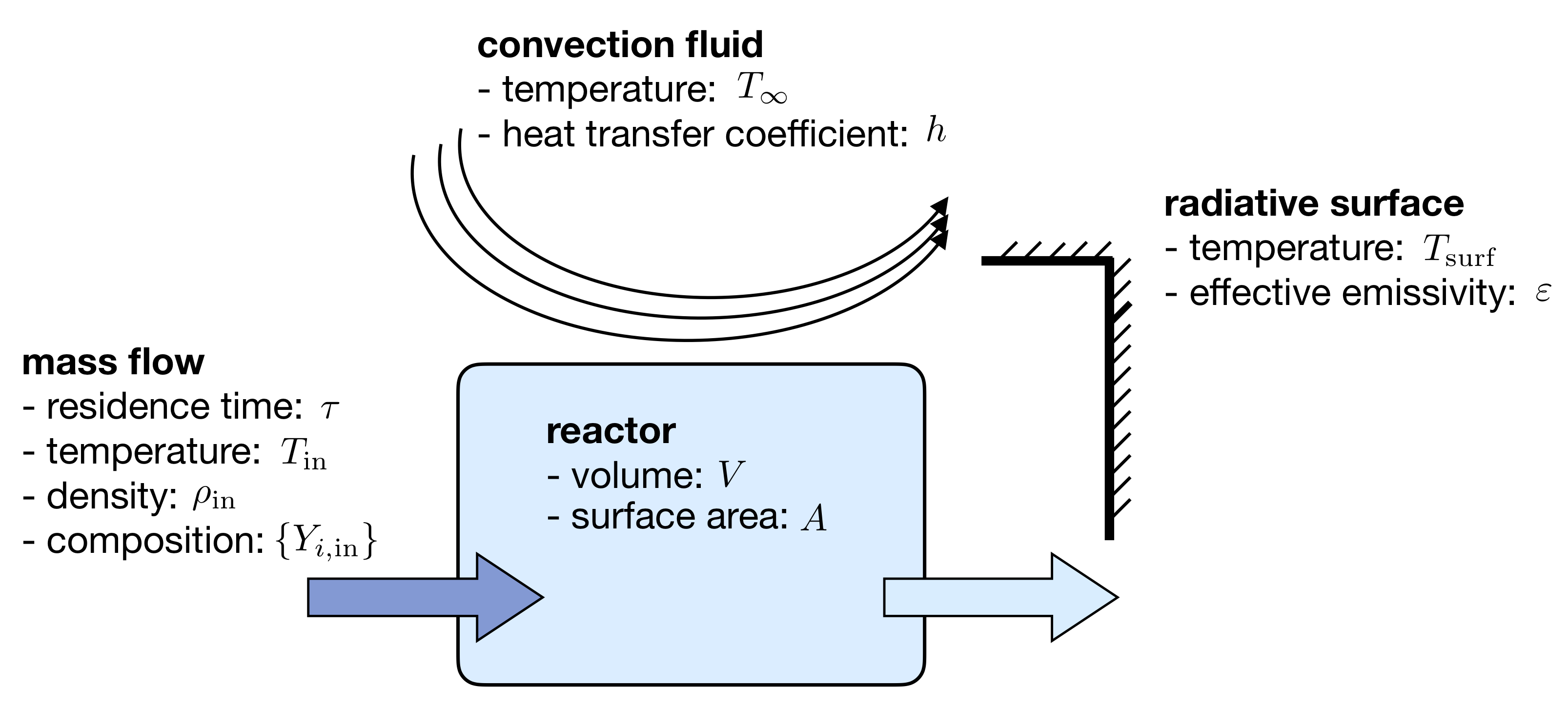
Fig. 1.1 Isochoric reactor with mass transfer and convective and radiative heat transfer
Isochoric reactors are governed by the following equations for the reactor density, temperature, and first \(n-1\) mass fractions. \(\omega_i\) is the net mass production rate of species \(i\) due to chemical reactions, \(c_v\) is the specific, isochoric heat capacity of the mixture, and \(e_i\) and \(e_{i,\mathrm{in}}\) are the specific internal energy of species \(i\) in the feed and reactor. \(\sigma\) is the Stefan-Boltzmann constant. We solve these equations in Spitfire to maximize sparsity and minimize calculation cost of Jacobian matrices. Recent work [MJ2018] has shown that the conservation error that results from solving a temperature equation instead of an energy equation is negligible when high-order time integration methods such as those in Spitfire are used. Closed reactors are obtained by setting \(\tau\to\infty\). Adiabatic reactors are obtained by setting \(h,\varepsilon\to0\). Isothermal reactors are obtained by setting the entire right-hand side of the temperature equation to zero.
Michael A. Hansen, James C. Sutherland, On the consistency of state vectors and Jacobian matrices, Combustion and Flame, Volume 193, 2018, Pages 257-271
1.1.6. Isobaric Reactors
Figure Fig. 1.2 diagrams an open, constant-pressure reactor with diathermal walls. The pressure, \(p\), of this reactor is held constant by the motion of a weightless, frictionless piston. The expansion work done by this process is an important difference between isobaric and isochoric reactors. We solve the following equations governing isobaric reactors. \(c_p\) is the specific, isobaric heat capacity of the mixture, and \(h_i\) and \(h_{i,\mathrm{in}}\) are the specific internal enthalpy of species \(i\) in the feed and reactor.
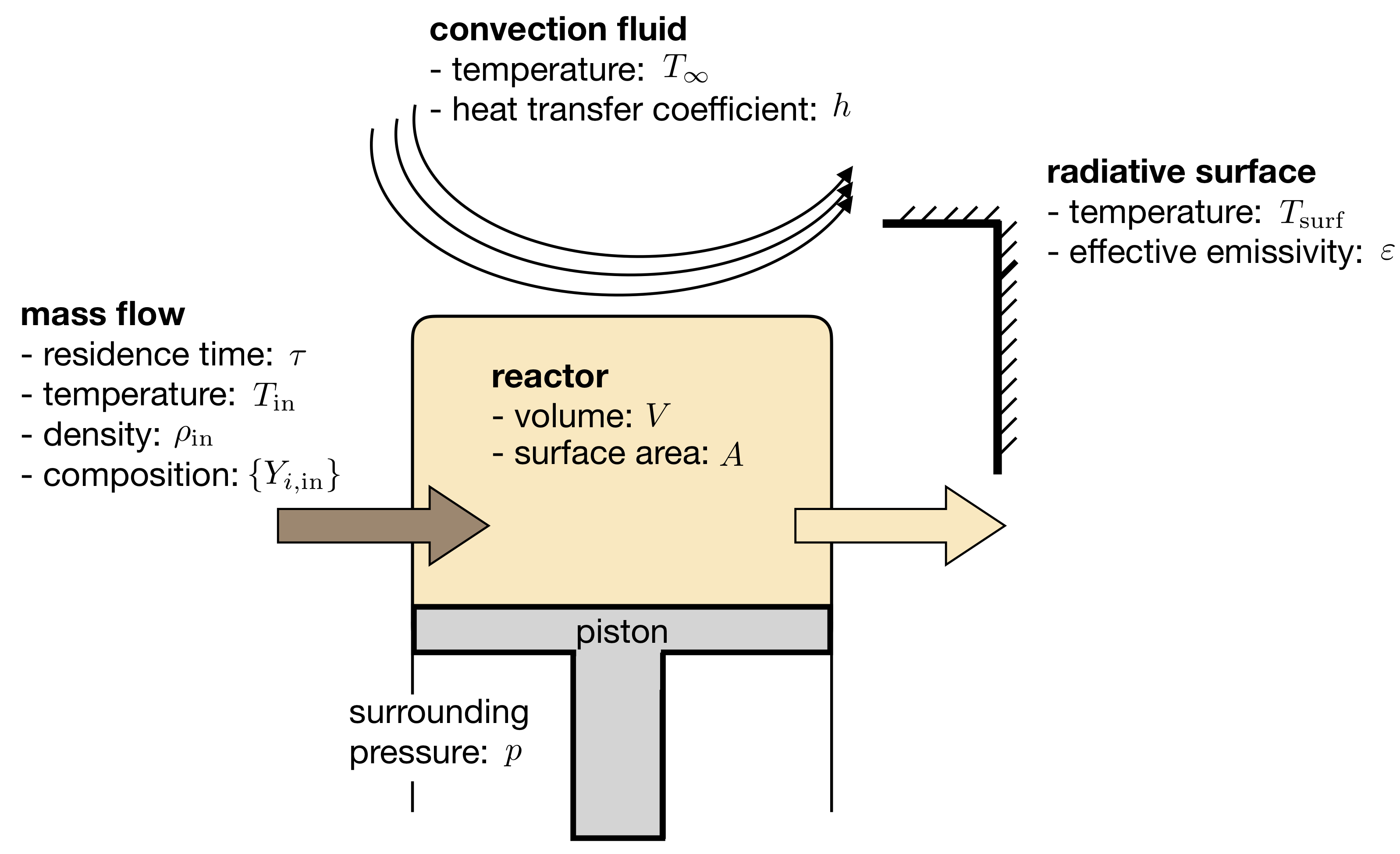
Fig. 1.2 Isobaric reactor with expansion work, mass transfer, and convective and radiative heat transfer
1.1.7. Chemical Kinetic Models
Spitfire currently supports various forms of reaction rate expressions for homogeneous gas-phase systems. Let \(n_r\) be the number of elementary reactions. The net mass production rate of species \(i\) is then
where \(\nu_{i,j}\) is the net molar stoichiometric coefficient of species \(i\) in reaction \(j\) and \(q_j\) is the rate of progress of reaction \(j\).
The rate of progress is decomposed into two parts: first, the mass action component \(\mathcal{R}_j\), and second, the TBAF component \(\mathcal{C}_j\) which contains third-body enhancement and falloff effects.
The mass action component consists of forward and reverse rate constants \(k_{f,j}\) and \(k_{r,j}\) along with products of species concentrations \(\left\langle c_k\right\rangle\),
in which \(\nu^f_{i,j}\) and \(\nu^r_{i,j}\) are the forward and reverse stoichiometric coefficients of species \(i\) in reaction \(j\), respectively.
The forward rate constant is found with a modified Arrhenius expression,
where \(A_j\), \(b_j\), and \(E_{a,j}\) are the pre-exponential factor, temperature exponent, and activation energy of reaction \(j\), respectively. We define \(T_{a,j}=E_{a,j}/R_u\) as the activation temperature.
The reverse rate constant of an irreversible reaction is zero. \(k_{r,j}\) for a reversible reaction is found with the equilibrium constant \(K_{c,j}\), via \(k_{r,j} = k_{f,j}/K_{c,j}\). The equilibrium constant is
where \(\Xi_j=\sum_{k=1}^{N}\nu_{k,j}\) and \(B_k\) is
For the TBAF component \(\mathcal{C}_j\) there are two nontrivial cases: (1) a three-body reaction and, (2) a unimolecular/recombination falloff reaction. If a reaction is not of a three-body or falloff type, then \(\mathcal{C}_j = 1\). For three-body reactions, it is
where \(\alpha_{i,j}\) is the third-body enhancement factor of species \(i\) in reaction \(j\), and \(\left\langle c_{TB,j}\right\rangle\) is the third-body-enhanced concentration of reaction \(j\). The quantity \(\alpha_{i,j}\) defaults to one if not specified. For falloff reactions, the TBAF component is
in which \(p_{fr,j}\) and \(\mathcal{F}_j\) are the falloff reduced pressure and falloff blending factor, respectively. The falloff reduced pressure is
where \(k_{0,j}\) is the low-pressure limit rate constant evaluated with low-pressure Arrhenius parameters \(A_{0,j}\), \(b_{0,j}\), \(E_{a,0,j}\), and \(\mathcal{T}_{F,j}\) is the concentration of the mixture which is either that of a single species if specified or the third-body-enhanced concentration if not.
The falloff blending factor \(\mathcal{F}_j\) depends upon the specified falloff form. For the Lindemann approach, \(\mathcal{F}_j = 1\). In the Troe form,
where \(a_{\text{Troe}}\), \(T^{*}\), \(T^{**}\), and \(T^{***}\) are specified parameters of the Troe form. If \(T^{***}\) is unspecified in the mechanism file then its term is ignored.
todo: add description of new non-elementary reaction rates
1.1.8. Species Thermodynamics
Spitfire supports ideal mixtures of thermally perfect species, and species heat capacity may be modeled as a constant or through a NASA-7 or NASA-9 polynomial. NASA-7 polynomials must be used with two temperature regions, while any number of regions may be used with a NASA-9 polynomial.
1.2. Tutorials
- 1.2.1. Setting up Thermochemistry Calculations with Cantera and Spitfire
- 1.2.2. One-step Ignition Mechanism for n-heptane/air Combustion
- 1.2.3. Ignition Delay Profiles for a Two-Stage Ignition Fuel
- 1.2.4. A Time-Dependent Flow Reactor: Periodic Ignition/Extinction
- 1.2.5. Explosive Mode Analysis of Isothermal vs Adiabatic Reactors
- 1.2.6. Steady State Multiplicity in n-heptane/air Mixtures
- 1.2.7. Introduction to Flamelet Models & Spitfire
- 1.2.8. Tabulation API Example: Adiabatic Flamelet Models
- 1.2.9. Tabulation API Example: Nonadiabatic Flamelet Models
- 1.2.10. Tabulation API Example: Superadiabatic Flamelet Models
- 1.2.11. Tabulation API Example: Methane Shear Layer
- 1.2.12. Transient Flamelet Example: Ignition and Advanced Time Integration
- 1.2.13. Transient Flamelet Example: Ignition Sensitivity to Rate Parameter
- 1.2.14. Custom Tabulation Example: 4D Coal Combustion Model