2. Chemical Reaction Models

Demonstrations:

• 2.1. Setting up Thermochemistry Calculations with Cantera and Spitfire
• 2.2. One-step Ignition Mechanism for n-heptane/air Combustion
• 2.3. Ignition Delay Profiles for a Two-Stage Ignition Fuel
• 2.4. A Time-Dependent Flow Reactor: Periodic Ignition/Extinction
• 2.5. Explosive Mode Analysis of Isothermal vs Adiabatic Reactors
• 2.6. Steady State Multiplicity in n-heptane/air Mixtures
• 2.7. Introduction to Flamelet Models & Spitfire
• 2.8. Tabulation API Example: Adiabatic Flamelet Models
• 2.9. Tabulation API Example: Nonadiabatic Flamelet Models
• 2.10. Tabulation API Example: Presumed PDF SLFM Tables
• 2.11. Custom Presumed PDF: log-mean PDF of the scalar dissipation rate
• 2.12. Tabulation API Example: Methane Shear Layer
• 2.13. Transient Flamelet Example: Ignition and Advanced Time Integration
• 2.14. Transient Flamelet Example: Ignition Sensitivity to Rate Parameter
• 2.15. Custom Tabulation Example: 4D Coal Combustion Model

The following sections detail some of the math behind Spitfire’s reaction modeling capabilities. We present the governing equations for non-premixed flamelets and homogeneous reactors, and supported reaction rate laws and thermodynamic property models.

2.16. Governing Equations for Non-premixed Flamelets

Spitfire’s flamelet and tabulation capabilities support generalized flamelet models for RANS/LES of hydrocarbon pool fires in the non-premixed combustion regime. While direct support is provided for sooting hydrocarbon fires, Spitfire leverages a modular, extensible stack from thermochemistry evaluator, numerical methods, solvers, and tabulation techniques. In this section we detail the governing equations solved by Spitfire for equilibrium, strained steady/transient, adiabatic/nonadiabatic flamelets. All of these equations are defined with the mixture fraction coordinate, which is a conserved scalar that describes inert mixing between fuel and air in a fire. These equations can be derived in a variety of ways, either through local coordinate transformations along the isosurfaces of the mixture fraction or by transforming species transport equations to follow a general Lagrangian coordinate frame. In both cases, time and length scale separation arguments lead to one-dimensional equilibrium/strained/nonadiabatic flamelet models of flows with two inlets.

The thermochemical state is described with the mass fractions \(Y_i\) and temperature \(T\). These are described by the mixture fraction \(\mathcal{Z}\) and other parameters, and in transient flamelets we consider evolution in a Lagrangian time \(t\). Equations (2.3) and (2.4) describe adiabatic flamelets, which balance molecular mixing (with strength proportional the scalar dissipation rate \(\chi\)) with species production/consumption and heat release through chemical reactions. These equations include variable heat capacity effects and the full form of the heat flux including the diffusive enthalpy temrs. They do not account for differential diffusion and are based on a unity Lewis number and mass fraction form of the species diffusive fluxes. Generalizations of the diffusive flux models have been derived and are planned for a future version of Spitfire. The variable heat capacity term and enthalpy flux terms are optional in Spitfire, but are included by default as they are very important for modeling nonadiabatic flows with strong coupling to radiative losses. The steady version of this equation set is derived by simply removing the time derivative term.

(2.3)\[\frac{\partial Y_i}{\partial t} = \frac{\chi}{2}\frac{\partial^2 Y_i}{\partial \mathcal{Z}^2} + \frac{\omega_i}{\rho},\]

(2.4)\[\frac{\partial T}{\partial t} = \frac{\chi}{2}\left(\frac{\partial^2 T}{\partial \mathcal{Z}^2} + \frac{\partial T}{\partial \mathcal{Z}}\sum_{i=1}^{n}\frac{c_{p,i}}{c_p}\frac{\partial Y_i}{\partial \mathcal{Z}} + \frac{1}{c_p}\frac{\partial c_p}{\partial \mathcal{Z}}\frac{\partial T}{\partial \mathcal{Z}}\right) - \frac{1}{\rho c_p}\sum_{i=1}^{n}\omega_i h_i.\]

These equations are supplemented by Dirichlet boundary conditions defined by the oxidizer and fuel states,

(2.5)\[\begin{split}T(t, 0) &= T_{\mathrm{oxy}}, \\ Y_i(t, 0) &= Y_{i,\mathrm{oxy}}, \\ T(t, 1) &= T_{\mathrm{fuel}}, \\ Y_i(t, 1) &= Y_{i,\mathrm{fuel}}.\end{split}\]

The dissipation rate \(\chi\) can be a constant or depend on the mixture fraction. Spitfire provides the common form due to Peters:

(2.6)\[\chi(\mathcal{Z}) = \chi_{\mathrm{max}} \exp\left( -2\left[\mathrm{erfinv}(2\mathcal{Z}-1)\right]^2 \right).\]

Spitfire also supports nonadiabatic flamelet models, which modifies only the temperature equation,

(2.7)\[\frac{\partial T}{\partial t} = \left.\frac{\partial T}{\partial t}\right|_{\mathrm{adiabatic}} + \frac{1}{\rho c_p}\left(h(T_\infty - T) + \varepsilon\sigma(T_\mathrm{surf}^4 - T^4)\right).\]

The convection and radiation coefficients and reference temperatures are allowed to vary over the mixture fraction. Further, the heat loss terms can be scaled to facilitate simulation of strong radiative quenching in large sooting fires,

(2.8)\[\frac{\partial T}{\partial t} = \left.\frac{\partial T}{\partial t}\right|_{\mathrm{adiabatic}} + \frac{1}{\rho c_p}\frac{\chi_{\mathrm{max}}}{\mathcal{Z}_{\mathrm{st}}(1 - \mathcal{Z}_{\mathrm{st}})}\left(h\frac{T_\infty - T}{T_{\mathrm{max}} - T_\infty} + \varepsilon\sigma\frac{T_\mathrm{surf}^4 - T^4}{T_{\mathrm{max}}^4 - T_\mathrm{surf}^4}\right).\]

where \(\mathcal{Z}_{\mathrm{st}}\) is the stoichiometric mixture fraction. The preferred model supported in Spitfire for hydrocarbon pool fires is to use a convective/linear form of the heat loss with \(h'\) to \(10^6-10^7\), which rapidly drives hydrocarbon flamelets to extinction, covering a wide range of the heat loss space broadly throughout the mixture fraction.

2.17. Governing Equations for Homogeneous Reactors

Homogeneous, or ‘zero-dimensional,’ reactor models represent well-mixed combustion systems wherein there are no spatial gradients in any quantity describing the chemical mixture. In such a system the temperature \(T\), pressure \(p\), and composition, expressed by the mass fractions \(\{Y_i\}\), are all homogeneous and a reactor may be modeled as a point in space whose properties vary only in time, \(t\). Zero-dimensional systems are idealizations of very complex systems but have their place in the modeling of combustion processes. In a lab setting this idealization can be approached with jet-stirred reactors (JSR, also commonly referred to as a continuous stirred tank reactor (CSTR), perfectly stirred reactor (PSR), and Longwell reactor) and rapid compression machines (RCM). A JSR is a continuous stirred tank reactor to which reactants are fed and mixed rapidly through several opposed jets. A JSR unit coupled with downstream gas chromatography and mass spectrometry can be used to quantify the composition of the chemical mixture as reaction proceeds. Detailed models of combustion kinetics are developed through comparison with experimental data from such systems. The rapid computational solution of kinetic models for simple, zero-dimensional reactors is of great fundamental importance to combustion modeling.

In Spitfire we model mixtures of ideal gases in twelve types of reactors distinguished by their configuration, heat transfer, and mass transfer. We use configuration to distinguish isochoric, or constant-volume, reactors from isobaric, or constant-pressure, ones. Mass transfer refers to a closed, or batch, reactor or an open reactor with mass flow at specified mean residence time. Three types of heat transfer are available:

• adiabatic: a reactor with insulated walls that allow no heat transfer with the surroundings

• isothermal: a reactor whose temperature is held exactly constant for all time

• diathermal: a reactor whose walls allow a finite rate of heat transfer by radiative heat transfer to a nearby surface and convective heat transfer to a fluid flowing around the reactor

Below we detail the equations governing isochoric and isobaric reactors with any pair of models for mass and transfer. In all cases, the gas is modeled as a mixture of thermally perfect gases. The ideal gas law applies to each species and the bulk mixture.

(2.9)\[p = \rho R_\mathrm{mix} T,\]

where the mixture specific gas constant, \(R_\mathrm{mix}\), is the universal molar gas constant divided by the mixture molar mass,

(2.10)\[M_\mathrm{mix} = \left(\sum_{i=1}^{n}\frac{Y_i}{M_i}\right)^{-1},\]

where \(M_i\) is the molar mass of species \(i\) in a mixture with \(n\) distinct species. Additionally, the mass fractions, of which only \(n-1\) are independent (and only \(n-1\) are solved for in Spitfire), are related by

(2.11)\[Y_n = 1 - \sum_{i=1}^{n-1}Y_i.\]

2.17.1. Isochoric Reactors

Figure Fig. 2.1 diagrams an open, constant-volume reactor with diathermal walls. The reactor has volume \(V\) and surface area \(A\). Convective heat transfer is described by a fluid temperature \(T_\infty\) and convective heat transfer coefficient \(h\). Radiative heat transfer is determined by the temperature of the surface, \(T_\mathrm{surf}\), and effective emissivity, \(\varepsilon\). Finally, for an isochoric reactor, mass transfer is specified by the residence time \(\tau\), based on volumetric flow rate, and inflowing state with temperature \(T_\mathrm{in}\), density \(\rho_\mathrm{in}\), and mass fractions \(\{Y_{i,\mathrm{in}}\}\).

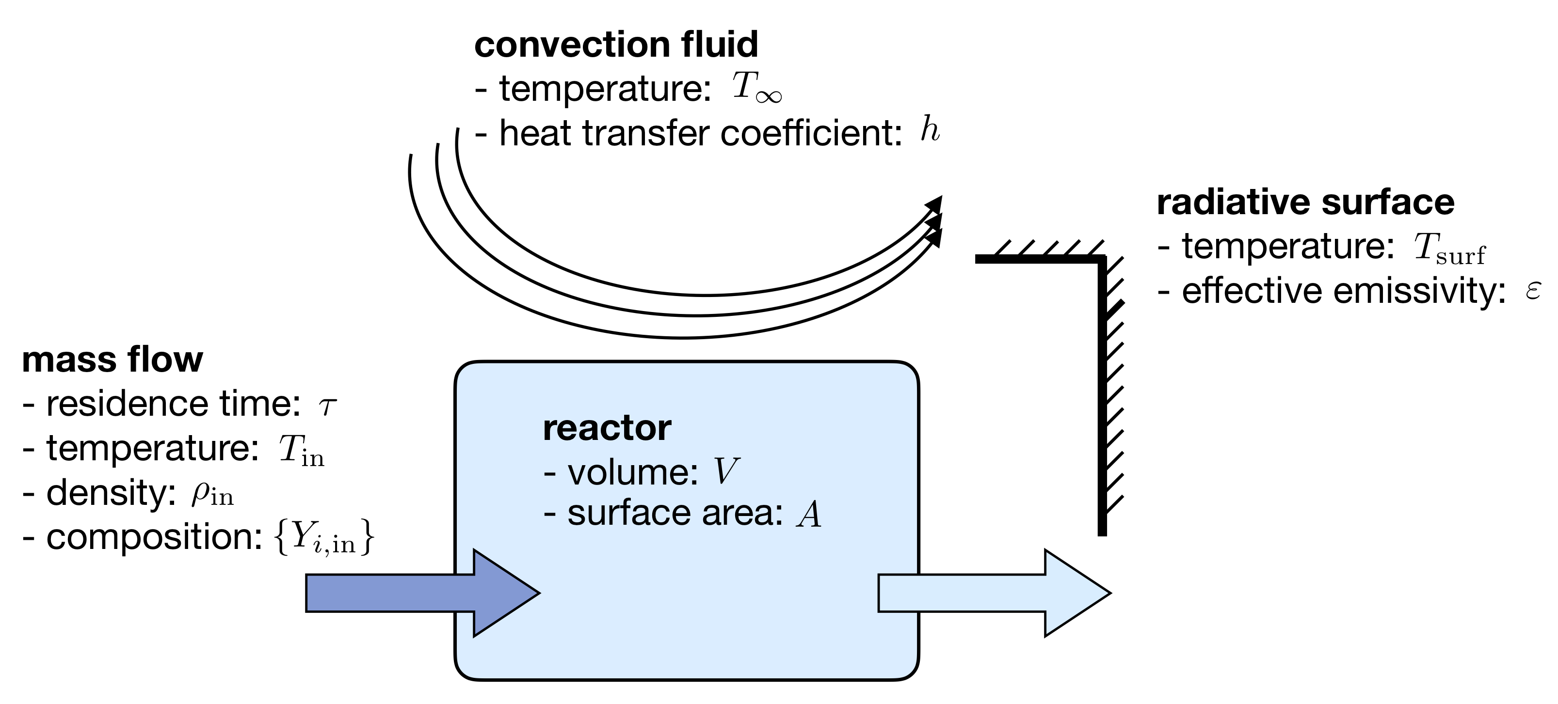
Fig. 2.1 Isochoric reactor with mass transfer and convective and radiative heat transfer

Isochoric reactors are governed by the following equations for the reactor density, temperature, and first \(n-1\) mass fractions. \(\omega_i\) is the net mass production rate of species \(i\) due to chemical reactions, \(c_v\) is the specific, isochoric heat capacity of the mixture, and \(e_i\) and \(e_{i,\mathrm{in}}\) are the specific internal energy of species \(i\) in the feed and reactor. \(\sigma\) is the Stefan-Boltzmann constant. We solve these equations in Spitfire to maximize sparsity and minimize calculation cost of Jacobian matrices. Recent work [MJ2018] has shown that the conservation error that results from solving a temperature equation instead of an energy equation is negligible when high-order time integration methods such as those in Spitfire are used. Closed reactors are obtained by setting \(\tau\to\infty\). Adiabatic reactors are obtained by setting \(h,\varepsilon\to0\). Isothermal reactors are obtained by setting the entire right-hand side of the temperature equation to zero.

(2.12)\[\frac{\partial \rho}{\partial t} = \frac{\rho_\mathrm{in} - \rho}{\tau},\]

(2.13)\[\frac{\partial Y_i}{\partial t} = \frac{\rho_\mathrm{in}}{\rho}\frac{Y_{i,\mathrm{in}} - Y_i}{\tau} + \frac{\omega_i}{\rho}, \quad i=1,\ldots,n-1\]

(2.14)\[\frac{\partial T}{\partial t} = \frac{\rho_\mathrm{in}}{\rho \tau c_v}\sum_{i=1}^{n}Y_{i,\mathrm{in}}(e_{i,\mathrm{in}} - e_i) - \frac{1}{\rho c_v}\sum_{i=1}^{n}\omega_i e_i + \frac{1}{\rho c_v}\frac{A}{V}\left(h(T_\infty - T) + \varepsilon\sigma(T_\mathrm{surf}^4 - T^4)\right),\]

MJ2018

Michael A. Hansen, James C. Sutherland, On the consistency of state vectors and Jacobian matrices, Combustion and Flame, Volume 193, 2018, Pages 257-271,

2.17.2. Isobaric Reactors

Figure Fig. 2.2 diagrams an open, constant-pressure reactor with diathermal walls. The pressure, \(p\), of this reactor is held constant by the motion of a weightless, frictionless piston. The expansion work done by this process is an important difference between isobaric and isochoric reactors. We solve the following equations governing isobaric reactors. \(c_p\) is the specific, isobaric heat capacity of the mixture, and \(h_i\) and \(h_{i,\mathrm{in}}\) are the specific internal enthalpy of species \(i\) in the feed and reactor.

(2.15)\[\frac{\partial Y_i}{\partial t} = \frac{Y_{i,\mathrm{in}} - Y_i}{\tau} + \frac{\omega_i}{\rho}, \quad i=1,\ldots,n-1\]

(2.16)\[\frac{\partial T}{\partial t} = \frac{1}{\tau c_p}\sum_{i=1}^{n}Y_{i,\mathrm{in}}(h_{i,\mathrm{in}} - h_i) - \frac{1}{\rho c_p}\sum_{i=1}^{n}\omega_i h_i + \frac{1}{\rho c_p}\frac{A}{V}\left(h(T_\infty - T) + \varepsilon\sigma(T_\mathrm{surf}^4 - T^4)\right),\]

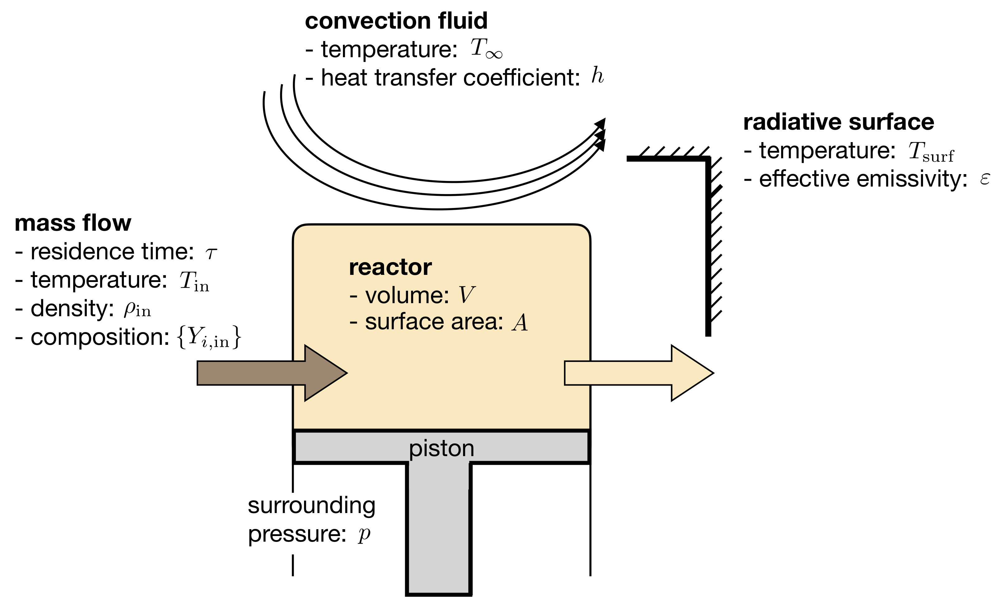
Fig. 2.2 Isobaric reactor with expansion work, mass transfer, and convective and radiative heat transfer

2.18. Chemical Kinetic Models

Spitfire currently supports various forms of reaction rate expressions for homogeneous gas-phase systems. Let \(n_r\) be the number of elementary reactions. The net mass production rate of species \(i\) is then

(2.17)\[\omega_i = M_i \sum_{j=1}^{n_r}\nu_{i,j}q_j,\]

where \(\nu_{i,j}\) is the net molar stoichiometric coefficient of species \(i\) in reaction \(j\) and \(q_j\) is the rate of progress of reaction \(j\).

The rate of progress is decomposed into two parts: first, the mass action component \(\mathcal{R}_j\), and second, the TBAF component \(\mathcal{C}_j\) which contains third-body enhancement and falloff effects.

(2.18)\[q_j = \overset{\text{mass action}}{\mathcal{R}_j}\cdot\overset{\text{3-body + falloff}}{\mathcal{C}_j}.\]

The mass action component consists of forward and reverse rate constants \(k_{f,j}\) and \(k_{r,j}\) along with products of species concentrations \(\left\langle c_k\right\rangle\),

(2.19)\[\mathcal{R}_j = k_{f,j}\prod_{k=1}^{N}\left\langle c_k\right\rangle^{\nu^f_{k,j}} - k_{r,j}\prod_{k=1}^{N}\left\langle c_k\right\rangle^{\nu^r_{k,j}},\]

in which \(\nu^f_{i,j}\) and \(\nu^r_{i,j}\) are the forward and reverse stoichiometric coefficients of species \(i\) in reaction \(j\), respectively.

The forward rate constant is found with a modified Arrhenius expression,

(2.20)\[k_{f,j} = A_j T^{b_j} \exp\left(-\frac{E_{a,j}}{R_u T}\right) = A_j T^{b_j} \exp\left(-\frac{T_{a,j}}{T}\right),\]

where \(A_j\), \(b_j\), and \(E_{a,j}\) are the pre-exponential factor, temperature exponent, and activation energy of reaction \(j\), respectively. We define \(T_{a,j}=E_{a,j}/R_u\) as the activation temperature.

The reverse rate constant of an irreversible reaction is zero. \(k_{r,j}\) for a reversible reaction is found with the equilibrium constant \(K_{c,j}\), via \(k_{r,j} = k_{f,j}/K_{c,j}\). The equilibrium constant is

(2.21)\[K_{c,j} = \left(\frac{p_\text{atm}}{R_u}\right)^{\Xi_j}\exp\left(\sum_{k=1}^{N}\nu_{k,j}B_k\right),\]

where \(\Xi_j=\sum_{k=1}^{N}\nu_{k,j}\) and \(B_k\) is

(2.22)\[B_k = -\ln(T) + \frac{M_k}{R_u}\left(s_k - \frac{h_k}{T}\right).\]

For the TBAF component \(\mathcal{C}_j\) there are two nontrivial cases: (1) a three-body reaction and, (2) a unimolecular/recombination falloff reaction. If a reaction is not of a three-body or falloff type, then \(\mathcal{C}_j = 1\). For three-body reactions, it is

(2.23)\[\mathcal{C}_j = \left\langle c_{TB,j}\right\rangle = \sum_{i=1}^{N}\alpha_{i,j}\left\langle c_i\right\rangle,\]

where \(\alpha_{i,j}\) is the third-body enhancement factor of species \(i\) in reaction \(j\), and \(\left\langle c_{TB,j}\right\rangle\) is the third-body-enhanced concentration of reaction \(j\). The quantity \(\alpha_{i,j}\) defaults to one if not specified. For falloff reactions, the TBAF component is

(2.24)\[\mathcal{C}_j = \frac{p_{fr,j}}{1 + p_{fr,j}}\mathcal{F}_j,\]

in which \(p_{fr,j}\) and \(\mathcal{F}_j\) are the falloff reduced pressure and falloff blending factor, respectively. The falloff reduced pressure is

(2.25)\[p_{fr,j} = \frac{k_{0,j}}{k_{f,j}}\mathcal{T}_{F,j},\]

where \(k_{0,j}\) is the low-pressure limit rate constant evaluated with low-pressure Arrhenius parameters \(A_{0,j}\), \(b_{0,j}\), \(E_{a,0,j}\), and \(\mathcal{T}_{F,j}\) is the concentration of the mixture which is either that of a single species if specified or the third-body-enhanced concentration if not.

The falloff blending factor \(\mathcal{F}_j\) depends upon the specified falloff form. For the Lindemann approach, \(\mathcal{F}_j = 1\). In the Troe form,

(2.26)\[\begin{split}\mathcal{F}_j &= \mathcal{F}_{\text{cent}}^{1/(1+(A/B)^2)}, \\ \mathcal{F}_{\text{cent}} &= (1-a_{\text{Troe}})\exp\left(-\frac{T}{T^{***}}\right) + a_{\text{Troe}}\exp\left(-\frac{T}{T^{*}}\right) + \exp\left(-\frac{T^{**}}{T}\right), \\ A &= \log_{10}p_{FR,j} - 0.67\log_{10}\mathcal{F}_{\text{cent}} - 0.4, \\ B &= 0.806 - 1.1762\log_{10}\mathcal{F}_{\text{cent}} - 0.14\log_{10}p_{FR,j},\end{split}\]

where \(a_{\text{Troe}}\), \(T^{*}\), \(T^{**}\), and \(T^{***}\) are specified parameters of the Troe form. If \(T^{***}\) is unspecified in the mechanism file then its term is ignored.

todo: add description of new non-elementary reaction rates

2.19. Species Thermodynamics

Spitfire supports ideal mixtures of thermally perfect species, and species heat capacity may be modeled as a constant or through a NASA-7 or NASA-9 polynomial. NASA-7 polynomials must be used with two temperature regions, while any number of regions may be used with a NASA-9 polynomial.